ct=c0+c1yt+c2ct-1
Using the data the following equation can be obtained:
ct = 0.1952 + 0.3486yt + 0.6364ct-1
Again we must look at whether this equation gives a satisfactory estimation of the consumption function. The simplest method of this is graphical although full statistical tests are included in the appendix. The top of figure 2 shows a very strong correlation between the actual consumption figures and the ones derived from our equation; however the bottom half still shows some large residual errors, especially in the late 1980’s although these errors are smaller than for our original equation.
Fig. 2
Another method of determining permanent income is to look at rational expectations. Consumers will predict their future incomes as accurately as possible using all information available to them at the time. This means that if a person was calculating their consumption for period t they would use all the information available to them up until that time. However this can be broken down into areas; information available at time t-1 and “new” information that came available between t-1 and t. The first of these should be reflected in ct-1. Rational expectation assumes that any “new” information has no relevance to information available at time t-1 or it would have been included in that calculation so this implies that the consumption function would be as follows:
ct=c1ct-1
If we input our data into this equation then we obtain the following consumption function:
ct=1.002ct-1
If c1 = 1 then this would be a random walk, i.e. a period where consumption was equally likely to rise or fall, depending on the error (new information) however as expected the c1 value is greater than one due to increasing levels of income over time, this could be for a number of reasons although inflation is an obvious one.
Inflation is guaranteed to have an effect on consumption as it changes the value of money over each time frame. Inflation erodes the value of debt meaning that those in debt (usually the corporate and government sectors) gain while those creditors (usually the private sector) lose out. However real disposable income doesn’t take this into account and so an inflation variable must be added to the consumption function. In this case we do not need a log or an index of inflation but can use the basic inflation rate; when this is added in the consumption function would look like:
ct=c0+c1yt+c2ct-1+c3πt
Using our data we can now estimate this consumption function:
ct = 0.2104 + 0.3306yt + 0.6541ct-1- 0.001826πt
It is visibly obvious now that the equation is far more complex than the original Keynesian consumption function however whether it is a better prediction of consumption remains to be seen. Statistically and graphically this equation is the most accurate one with an R² value of 0.998, meaning that there is a very strong correlation between our derived line and the line of actual consumption as can be seen in figure 3 below. However the lower graph shows the residuals left by the equation and from the mid-eighties to the mid-nineties there are still large errors left:
Fig. 3.
Before another variable is added, the format of the equation must be changed slightly. The problem with the consumption function is that economic theory suggests that two different levels of consumption would occur in the long-run and in the short-run. In the long-run ‘consumer theory suggests that….permanent income will be proportion to actual income, and hence consumption should be proportional to income.’ However in the short-run common sense tells us that this would not be the case because of unexpected events and basic human behaviour. In order to incorporate both of these points there is a mechanism known as the error correction mechanism. This involves taking both cases and saying that yes, in the long-run consumption will be proportional to income but in the short-run this will never actually occur due to exogenous factors; however consumers will, in the short-run, try to adjust consumption to the be proportional to income but this adjustment will be gradual and will re-adjust as circumstances dictate. This would lead us to a consumption function like the one below where s = yt – ct:
Δct=c0+c1Δyt+c2st-1+c3πt
From that we obtain the function:
Δct = 0.01062 + 0.6556Δyt + 0.1089st-1 - 0.001038πt
As you can see from the graph below, consumption functions like the one illustrated above were used to predict consumption with great success up until the mid 1980’s however they failed to predict the rapid decline in savings soon after that.
Fig. 4.
The main reason, it was argued, was that a combination of rapidly rising house prices and increased availability of credit meant that people had more wealth and so increased their consumption. The argument was based on the fact that because the price of people’s houses went up and being available to secure loans and equity against your property became easier people started to borrow more money and so increase their consumption accordingly. Because of this, to accurately predict consumption house prices needed to come into consideration. If we include them in our equation we obtain the following equation where HP stands for house prices:
Δct = 0.01342 + 0.4657Δyt + 0.07634st-1 - 0.001617πt + 0.0007924HPt
As you can see from comparing figures 4 (above) and 5 (below), by adding the HP variable the difference between the derived and the actual consumptions during the late 80’s and early nineties is much closer:
Fig. 5.
However there is still an unaccounted for gap during this period, another reason that was argued about why the original model fell apart was because uncertainty about future wage raises was falling. Throughout the 1980’s income levels had increased much more steadily than during the 1970’s and so people saved less for precautionary reasons, which meant that they had more disposable income and so increased their consumption accordingly. Uncertainty is not an easy variable to measure but for this project, uncertainty was taken as the ‘standard deviation over the previous four years of the growth of real personal income.’ This meant that our equation looks as follows:
Δct = c0+c1Δyt+c2st-1+c3πt+c4HPt+c5Ut
This left the derived consumption function as:
Δct = 0.02213 + 0.3729Δyt + 0.07338st-1 - 0.00179πt + 0.0009742HPt - 4.439x10⁻⁸Ut
As you can see from comparing figures 5 and 6 there is virtually no difference after adding this variable as the co-efficient of uncertainty this means that uncertainty is either being modelled incorrectly or the argument that it played a major in the change of consumption over the late 80’s was incorrect.
Fig. 6.
Conclusion:
The aim of this project was to start with the simplest of theoretical model for consumption, the Keynesian consumption function and derive an equation that although not perfectly true would give an accurate prediction for consumption based on data of the UK economy over the last 50 years. The top graph in figure 6 shows the actual consumption against predicted consumption derived from our equation. There is a reasonably good correlation between the two lines, with an R² value of 0.72, which considering that the equation is time-series is fairly high. However there are still some medium sized residuals left on the bottom graph, showing that the equation still needs work. Some aspects of this model are still very basic; for example the time lag system used is the most basic with only a couple of previous years being taken into consideration. Likewise this equation is based on total consumption in the economy where as if the equation were to used for actual predictions it would be broken down into different categories of consumables. The uncertainty variable that we calculated needs re-evaluating as it never appeared to impact the consumption function at all. Still the aim of the project was achieved as a reasonably accurate function was successfully estimated.
Bibliography:
Sloman, J., Economics, 5th Ed., FT Prentice Hall, 2004
Griffiths, A. & Wall, S., Applied Economics, 10th Ed., FT Prentice Hall, 2004
Backhouse, R.E., Chapter 2 - Consumption and Savings,
Appendix
EQ( 1) Modelling C by OLS (using es1162proj.in7)
The estimation sample is: 1948 to 2003
Coefficient Std.Error t-value t-prob Part.R^2
Constant 13529.4 2978. 4.54 0.000 0.2765
Yd 0.922396 0.007378 125. 0.000 0.9966
sigma 9008.74 RSS 4.38249908e+009
R^2 0.996557 F(1,54) = 1.563e+004 [0.000]**
log-likelihood -588.375 DW 0.49
no. of observations 56 no. of parameters 2
mean(C) 354108 var(C) 2.27308e+010
C = + 1.353e+004 + 0.9224*Yd
(SE) (2.98e+003) (0.00738)
EQ( 2) Modelling LC by OLS (using es1162proj.in7)
The estimation sample is: 1948 to 2003
Coefficient Std.Error t-value t-prob Part.R^2
Constant 0.727310 0.09323 7.80 0.000 0.5298
LY 0.940298 0.007325 128. 0.000 0.9967
sigma 0.0246616 RSS 0.0328424053
R^2 0.996734 F(1,54) = 1.648e+004 [0.000]**
log-likelihood 128.898 DW 0.339
no. of observations 56 no. of parameters 2
mean(LC) 12.688 var(LC) 0.179543
LC = + 0.7273 + 0.9403*LY
(SE) (0.0932) (0.00733)
*** Warning: diagonal elements of W'W are very small or very different.
Numerical accuracy is endangered, try rescaling the data.
Algebra code for es1162proj.in7:
Yd_2 = (Yd+lag(Yd,1)+lag(Yd,2))/3;
Algebra code for es1162proj.in7:
Yp = log(Yd_2);
EQ(11) Modelling LC by OLS (using es1162proj.in7)
The estimation sample is: 1952 to 2003
Coefficient Std.Error t-value t-prob Part.R^2
Constant 0.618081 0.1305 4.73 0.000 0.3096
Yp 0.950745 0.01023 92.9 0.000 0.9942
sigma 0.0307511 RSS 0.0472815354
R^2 0.99424 F(1,50) = 8630 [0.000]**
log-likelihood 108.29 DW 0.436
no. of observations 52 no. of parameters 2
mean(LC) 12.7383 var(LC) 0.157852
LC = + 0.6181 + 0.9507*Yp
(SE) (0.131) (0.0102)
EQ(12) Modelling LC by OLS (using es1162proj.in7)
The estimation sample is: 1952 to 2003
Coefficient Std.Error t-value t-prob Part.R^2
LC_1 0.636355 0.1137 5.60 0.000 0.3898
Constant 0.195196 0.1028 1.90 0.063 0.0685
LY 0.348639 0.1080 3.23 0.002 0.1753
sigma 0.0182007 RSS 0.0162319734
R^2 0.998022 F(2,49) = 1.236e+004 [0.000]**
log-likelihood 136.088 DW 0.849
no. of observations 52 no. of parameters 3
mean(LC) 12.7383 var(LC) 0.157852
LC = + 0.6364*LC_1 + 0.1952 + 0.3486*LY
(SE) (0.114) (0.103) (0.108)
PcGive Graphics saved to E:\eq4.gwg
PcGive Graphics saved to E:\eq4.emf
EQ(13) Modelling LC by OLS (using es1162proj.in7)
The estimation sample is: 1952 to 2003
Coefficient Std.Error t-value t-prob Part.R^2
LC_1 1.00214 0.0002142 4678. 0.000 1.0000
sigma 0.0196467 RSS 0.0196856845
log-likelihood 131.072 DW 1.24
no. of observations 52 no. of parameters 1
mean(LC) 12.7383 var(LC) 0.157852
LC = + 1.002*LC_1
(SE) (0.000214)
PcGive Graphics saved to E:\eq5.gwg
PcGive Graphics saved to E:\eq5.emf
EQ(14) Modelling LC by OLS (using es1162proj.in7)
The estimation sample is: 1952 to 2003
Coefficient Std.Error t-value t-prob Part.R^2
LC_1 0.654142 0.09933 6.59 0.000 0.4747
Constant 0.210448 0.08977 2.34 0.023 0.1027
LY 0.330610 0.09436 3.50 0.001 0.2037
Inf -0.00182602 0.0004513 -4.05 0.000 0.2543
sigma 0.0158794 RSS 0.0121035216
R^2 0.998525 F(3,48) = 1.083e+004 [0.000]**
log-likelihood 143.718 DW 0.883
no. of observations 52 no. of parameters 4
mean(LC) 12.7383 var(LC) 0.157852
LC = + 0.6541*LC_1 + 0.2104 + 0.3306*LY - 0.001826*Inf
(SE) (0.0993) (0.0898) (0.0944) (0.000451)
Means
DLC Constant DLY Inf S_1
0.026250 1.0000 0.027993 5.9691 0.031910
Standard Deviations
DLC Constant DLY Inf S_1
0.019951 0.00000 0.021134 4.8543 0.036799
Correlation matrix
DLC Constant DLY Inf S_1
DLC 1.0000
Constant 0.00000 0.00000
DLY 0.74022 0.00000 1.0000
Inf -0.47105 0.00000 -0.36329 1.0000
S_1 -0.00049433 0.00000 -0.22889 0.16807 1.0000
EQ( 1) Modelling DLC by OLS (using es1162proj.in7)
The present sample is: 1949 to 2003
Descriptive statistics
DLC = +0.01062 +0.6556 DLY -0.001038 Inf
(SE) ( 0.004535) ( 0.08744) (0.0003759)
+0.1089 S_1
( 0.04746)
R^2 = 0.632903 F(3,51) = 29.309 [0.0000] \sigma = 0.0124386 DW = 1.29
RSS = 0.007890707309 for 4 variables and 55 observations
Seasonal means of differences are
0.00013
R^2 relative to difference+seasonals = 0.69974
AR 1- 2 F( 2, 49) = 4.9335 [0.0112] *
ARCH 1 F( 1, 49) = 4.7432 [0.0343] *
Normality Chi^2(2)= 5.0768 [0.0790]
Xi^2 F( 6, 44) = 0.72456 [0.6321]
Xi*Xj F( 9, 41) = 0.58121 [0.8046]
RESET F( 1, 50) = 0.089081 [0.7666]
Descriptive statistics
Means
DLC Constant DLY Inf S_1 HP_Inf
0.026250 1.0000 0.027993 5.9691 0.031910 8.8491
Standard Deviations
DLC Constant DLY Inf S_1 HP_Inf
0.019951 0.00000 0.021134 4.8543 0.036799 8.6500
Correlation matrix
DLC Constant DLY Inf S_1
DLC 1.0000
Constant 0.00000 0.00000
DLY 0.74022 0.00000 1.0000
Inf -0.47105 0.00000 -0.36329 1.0000
S_1 -0.00049433 0.00000 -0.22889 0.16807 1.0000
HP_Inf 0.46519 0.00000 0.39641 0.22712 0.10990
HP_Inf
HP_Inf 1.0000
EQ( 2) Modelling DLC by OLS (using es1162proj.in7)
The present sample is: 1949 to 2003
DLC = +0.01342 +0.4657 DLY -0.001617 Inf
(SE) ( 0.004141) ( 0.09411) (0.0003727)
+0.07634 S_1 +0.0007924 HP_Inf
( 0.04351) (0.0002169)
R^2 = 0.710259 F(4,50) = 30.642 [0.0000] \sigma = 0.0111606 DW = 1.49
RSS = 0.006227953112 for 5 variables and 55 observations
Seasonal means of differences are
0.00013
R^2 relative to difference+seasonals = 0.76301
AR 1- 2 F( 2, 48) = 2.5038 [0.0924]
ARCH 1 F( 1, 48) = 0.1878 [0.6667]
Normality Chi^2(2)= 0.39869 [0.8193]
Xi^2 F( 8, 41) = 0.54099 [0.8186]
Xi*Xj F(14, 35) = 0.53082 [0.8976]
RESET F( 1, 49) = 0.14221 [0.7077]
---- PcGive 9.10 session started at 19:53:05 on Sunday 24 April 2005 ----
Descriptive statistics
Means
DLC Constant S_1 DLY HP_Inf U
0.026440 1.0000 0.034970 0.028037 8.9811 16790.
Inf
6.0830
Standard Deviations
DLC Constant S_1 DLY HP_Inf U
0.020282 0.00000 0.033813 0.021528 8.7545 21894.
Inf
4.9098
Correlation matrix
DLC Constant S_1 DLY HP_Inf
DLC 1.0000
Constant 0.00000 0.00000
S_1 -0.025510 0.00000 1.0000
DLY 0.74051 0.00000 -0.25974 1.0000
HP_Inf 0.46981 0.00000 0.086457 0.40063 1.0000
U -0.30424 0.00000 -0.15604 -0.29136 0.063056
Inf -0.48217 0.00000 0.12881 -0.36765 0.22112
U Inf
U 1.0000
Inf 0.081866 1.0000
EQ( 3) Modelling DLC by OLS (using es1162proj.in7)
The present sample is: 1953 to 2003
DLC = +0.02213 +0.07338 S_1 +0.3729 DLY
(SE) ( 0.005464) ( 0.059) ( 0.1046)
+0.0009742 HP_Inf -0.00179 Inf -4.439e-007 U
(0.0002279) (0.0003766) (1.89e-007)
R^2 = 0.720782 F(5,45) = 23.233 [0.0000] \sigma = 0.0108564 DW = 1.59
RSS = 0.005303797832 for 6 variables and 51 observations
Seasonal means of differences are
-0.00039
R^2 relative to difference+seasonals = 0.76502
AR 1- 2 F( 2, 43) = 1.5488 [0.2241]
ARCH 1 F( 1, 43) = 0.025411 [0.8741]
Normality Chi^2(2)= 0.13477 [0.9348]
Xi^2 F(10, 34) = 0.71796 [0.7019]
Xi*Xj F(20, 24) = 0.73126 [0.7595]
RESET F( 1, 44) = 0.20253 [0.6549]
Keynes, John Maynard, Extracted from Sloman, J., Economics, 5th Ed., FT Prentice Hall, 2004 pg304.
Sloman, J., Economics, 5th Ed., FT Prentice Hall, 2004 pg 467
Backhouse, R.E., Consumption and Savings, pg32-33
Backhouse, R.E., Consumption and Savings, pg36