This method ensures that I have a fair proportion of data from each “strata” (Year 7 form). I chose this method because of the fair representation it gives. Cluster sampling is limited in class sizes this small, as will be too biased. I also attempted systematic sampling, where every nth piece of data is used, but I experienced many problems with this. For example, if I took every 4th piece of data, sometimes the data I should have used was inadequate, as it was incomplete (etc). This meant that I had to choose the next piece of data, which messed up the system, and I often did not have enough pieces of data in the end.
To display this information, a scatter graph should be used. A scatter graph can be used to show the distance the shot putt was thrown, against the distance the discus was thrown. If shot is placed on the x-axis, one can say:
“If one can throw the shot x metres, they can throw the discus y metres.”
Looking at the relationship shown on the scatter graph can prove this kind of statement. The graph clearly shows that there is positive correlation between the two events. This means, that as the results for shot increase, so do the results for discus.
A line of best fit can be drawn, which should go through the mean (x, y). X, Y is found by finding the sum of the shot event and dividing by the total sample size (X). Then we find the sum of the discus event and divide by the total sample size (Y):
This means that X, Y is 5.2, 12.5. A gradient triangle can also seen on the graph:
Y 16.15 – 12.00 = 4.15
X 7.00 – 5.00 = 2.00
4.15 = 2.075 gradient
2.00
This means that for every 1m shot thrown, the discus is thrown 2.075m. The two cumulative frequency graphs, which I have produced, prove this, as if you time
any point on the shot graph by 2.075, you will get a point which can be found on the discus graph’s curve.
To extend my hypothesis, I will study the shot putt and discus a year 10 class, and a year 9 class, to see if they can throw any better. I will plot a scatter graph, and be able to tell whether there is any improvement from the gradient.
I expect that the year 10 and year 9 results will be better than the year 7’s results, as (in general) they will be taller, possibly be better at throwing as they would have had more practice. These factors should help the same pupils to be able to throw further in year 10 than in year 7.
As before with my scatter graph, I will plot 26 results, on the same size scale, for ease when comparing the two gradients.
Like the original scatter graph, the scatter graph, which depicts the results from year 9 and 10, also shows positive correlation. The mean is found as before (see back of graph):
Shot mean = 170.1461 = 6.54
26
Discus mean = 345.71 = 13.3
26
This helps to draw the line of best fit. This means the value of (x , y) is (6.54, 13.3). A gradient triangle can now be drawn for this graph and again the gradient can be worked out. It will also be positive, as the correlation is positive.
Y = 10.2 – 6 = 4.2
X = 5 – 3 = 2
4.2 = 2.1
2
This means that for every 1m that a year 10/9 can throw the shot putt, they can throw the discus 2.1m. This suggests that the pupils are better at throwing when they are in year 10/9, although there is not much difference in the two gradients.
Despite the small difference in gradients, there is a large difference in means:
This shows that extrapolation of the data for the rest of year 10 and year 9 must have effected the results heavily, if the mean for my results was more than the gradient. This could also show that there has been a mistake in my calculations, and is something to think about in regards to improvements.
The results also do not show us what the performance of year 8s was like, and makes it likely that extrapolation will effect the results which are portrayed on the graphs.
It is possible that the pupils’ throwing performance peaked in year 8 or that either of these graphs is not representative for all the year groups. It is also quite possible that their technique of throwing does not improve at all, as usually, there is only one lesson for discus and shot in an entire year, and the girls are only taught the technique in year 7, and expected to remember it after that. It is also possible that the data was entered incorrectly into the spreadsheet or was only half entered into either the spreadsheet or the initial sheet. This would have some effect on the mean and can throw off the graph.
Hypothesis Two – AS PUPILS GET OLDER, THEY GET BETTER AT LONG JUMP
I hypothesise that as pupils get older, they will be able to jump farther. This is because (generally) legs will have grown longer. This will improve the run up to the jump, which improves the jump itself. Theoretically, it will also mean that the actual jump should be easier because their legs will be longer, and they would have to put less effort into the jump. They will also have had more practice at jumping since the previous year.
For this hypothesis, I will display the data using histograms. I will do this, because histograms can display continuous data, showing the skew and the distribution clearly. It also means the sample sizes do not need to be the same as the y-axis is based on the frequency density.
The midpoints of the bars can also be joined up to produce a frequency polygon, which shows the skew even more clearly. I have data for three forms from year 7 to 10 (7H, 7S, 7V) and I will use all of the data (where possible) in the histograms, in an attempt to make my histograms more accurate.
This means that the concentration will be on classes as a whole, and not just the improvement of an individual. To find the frequency density, which will be on the y-axis of the histogram, the frequency needs to be divided by the class width.
e.g. 3 = 4
0.75
I will draw each of the histograms using the same scale so it is easier to compare them. The skew shown by the frequency polygon is fairly similar for each histogram but there are some differences. All four of the years have negative skew. The skew in years 9 and 10 is more negative than the previous years, which shows that the majority of lengths jumped are longer lengths. The number of longer lengths also increases in these years.
This proves my hypothesis that as you get older; your ability to compete in long jump improves. Standard deviation is used to show how the data is distributed about the mean. To find the mean, all the data is added up and divided by the number of pupils:
Total long jump distance = 205.96m
205.96 = 2.783243m
74
The standard deviation of the data can be worked out using the following formula: ∑(x –x)2
n
This shows how the data is spread in relation to the mean.
(2.15 – 2.70)2 + (2.16 – 2.70)2 + (2.17 – 2.70)2 etc.
74
= 0.3025 + 0.2916 + 0.2809 etc.
74
= 37.89871
74
= 0.512145m
The mean and standard deviation are in metres and have been rounded to three decimal places for ease. The standard deviations show that the data for year 8 is the most widely spread and the data for year 9 is the closest together.
The highest mean is for year 9 and the smallest standard deviation is also for year 9. This means that year 9 peaked in long jump. This may not be true for all the girls shown in the histograms or even for all girls, but the general population.
The lowest mean was for year 7, but this did not have the highest standard deviation. Year 8 has the highest standard deviation. Both year 7 and 8 have fairly similar performances (2.70m and 2.78m). This shows that their jumping ability did not really improve in these years. This seems quite likely, as there is only one hour lesson in a year for long jump for the girls to perform in, and you can not expect girls to improve so much then.
The histograms are also fairly similar for year 9 and year 10, but year 9’s results are a little better, as they are more negatively skewed. This also shows that the performance that peaked in year 9 slowly decreases in year 10.
Hypothesis Three – AS PUPILS GET OLDER, THEY GET BETTER AT SPRINTING THE 100M
I hypothesise that pupils will be able to sprint faster as they progress through the school. It is possible that some will have developed a keenness for running and so they will have practised more. They might have improved because they will have run more, or because they will be growing and so their legs will become longer, giving them a longer stride so that they will be able to run faster. This would enable them to improve their technique and give them an opportunity to become fitter.
I will use a sample size of 31 as this enables the median and the two quartiles to be easily located. To display this information I will use a cumulative frequency curve. This enables the median, the lower and upper quartiles and the inter-quartile range to be found easily.
I will use the data for anyone whose data is available, giving each remaining girl in the three year 7 forms a number between 1 and 64. I will then use a calculator again to generate 31 random numbers as before. I can then put the times from these pupils into tables and work out the frequency and then the cumulative frequency by adding the frequencies together. The group values are in seconds.
I drew the cumulative frequency curves on the same axis. This ensured that they could be easily compared. To work out the median values, one must be added to the total frequency and then divided by two to find the median. The median can be halved to find the lower quartile. Then, to find the upper quartile, the lower quartile id multiplied by three.
17 + 1 = 18
18 = 9, so the median is the 9th value
2
18 = 4.5, so the lower quartile is the 4.5th value
4
4.5 x 3 = 13.5, so the upper quartile is the 13.5th value.
I can then find the median and quartile values by drawing a line across at 9 for the median, 4.5 for the lower quartile and 13.5 for the upper quartile on the y-axis.
Where these lines meet the curves, a vertical line should be inserted. This will give the values for the median and the two quartiles. The inter-quartile range can be found by subtracting the lower quartile from the upper quartile. The inter-quartile range is not affected by extreme values.
To work out if there are any outliers for the box plots, the IQR must be multiplied by 1.5 and then added to the upper quartile, then subtracted from the lower quartile. Any data, which is not within this range, is called an outlier. Outliers are extreme values that can influence the mean of a set of data by making it lower or higher. Their effect can be seen on the Standard Deviation.
The cumulative frequency curves show that the times do not vary greatly between the years. The year 8s and 9s have the fastest running times however, they also have some of the slowest times. Year 7 and year 10 have roughly the same median and year 8 and 9 also have similar medians. Both years 8 and 7 show fairly normal skew, and Year 9 has definite positive skew. Year 10 has slight positive skew, and the IQR for year 10 is also the largest, which shows that the spread of times is greater in this year than in the others. For Year 8, the IQR is smallest for year 8, showing that their times are less spread and that there is less difference in between individuals’ performances. Year 7 has the slowest time. Year 9 has the fastest time as well as the only time below the lowest boundaries.
This hypothesis, like my last one suggests that the athletic peak for a pupil be during year 9. This may be biased for the dozens of reasons outlined in the introduction. We have no idea how the results would vary in a non-selective mixed school, non-selective boys/girls schools; selective mixed school or a selective boy’s school. It would also differ greatly from a school that focused more on sport.
One of the logical reasons for why the athletic peak may be in year 9, is that apart from year 10s, they are the eldest, and the Year 10s are under so much more pressure due to GCSE work, leaving less time for sport, etc.
It also possibly means that year 10s cannot concentrate as much when they are doing athletics because of the pressure of coursework. It is also possible that this year is not representative of other years that may continue getting better. There is however, only a certain amount that a teenager can improve before they reach the best of their ability and can only stay the same or get worse. This was referred to as the “peak” and achieved by most in CCHS during year 9.