Therefore it is clear that the error bounds for this root are [-0.5321, -0.5320] as such the solution is –0.55325 and the maximum error is +0.00005 or –0.00005.
[2,3]
Therefore it is clear that the error bounds for this root are [2.8793, 2.8794] as such the solution is 2.87935 and the maximum error is +0.00005 or –0.00005.
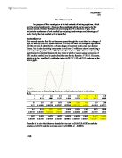
However in a number of cases the change of sign method will not work as shown below.
This method also does not work when there are several roots, which are extremely close together. In this case it will often only pick up one of the roots. There are also problems when there is a discontinuity in f(x). For example the function 1/x +2.6 has no root which is made clear in the below graph. Instead they converge to the false root highlighted by the dotted line.
Newton-Raphson
This method works on the theory that “the tangent to a curve can be used to obtain improved approximations to a root of an equation f(x)=0.” (A-level & As level mathematics, Longman revise guides.) This is a fixed-point estimation method as it is necessary to use an estimate of the root as a starting point. An estimate of x1 for a root or f(x)=0 is made and then the tangent to the curve y=f(x) at the point (x1,f(x1)) is drawn. The point at which the tangent crosses the x-axis gives the next approximation for the root and the process can then be repeated until the required degree of accuracy has been reached (shown on enlarged graph.) Therefore this method can be used to find the roots for the function x3-4x2+2x+2 as is shown below.
The general formula for Newton-Raphson is xn+1 = xn –f(x)
F’(x)
This formula will be used to find the roots for this function as shown below. Once this method has been used decimal search can be used to find the interval which the root lies in.
[-1,0] x1 = 0
x2 = -1 this is the root for this interval as the curve passes directly through –1.
[1,2] x1 = 1
x2 = 1.3
x3 = 1.31
x4 = 1.311 this is the root for this interval to three decimal places.
This shows that the error bounds for this root are [1.311, 1.312] making the solution 1.3115and therefore the maximum error is +0.0005 or –0.0005
[3,4] x1 = 4
x2 = 3.4
x3 = 3.22
x4 = 3.171 this is the root for this interval to three decimal places.
This shows that the error bounds for this root are [3.17, 3.171] making the solution 3.1705 and therefore the maximum error is +0.0005 or –0.0005
There are problems when using this method, for example poor choice of starting point means that there will be no convergence to the root. Also the method will not be successful if the function is discontinuous.
Rearranging the equation f(x)=0 into the form x=g(x)
This method works on the basis that “any value of x for which x=g(x) is clearly a root of the original equation (f(x)=0).”(Pure Mathematics 2, Hodder&Stoughton) To find a root the graphs y=x and y=g(x) are plotted, the points at which the two curve cross are the roots. The roots can then be found using the following method:
-
Make an estimate of the value of x1
-
Find the corresponding value of g(x1)
-
The value found for g(x1) should be taken to be the new estimate for x2
- This process can be repeated until the desired degree of accuracy has been reached.
The way this works is shown on the enlarged graph below.
This method is to be used to find the roots of x3-4x+1.
The formula can be rearranged into the form x=x3+1/4 which can then be plotted against x and using the above method it is possible to find the roots, using the iterative formula shown below.
xn+1 = xn3+1
4
[0,1] x1 = 1
x2 = 0.5
x3 = 0.28125
x4 = 0.255562
x5 = 0.254173
x6 = 0.254105
x7 = 0.254102
Therefore the root correct to four decimal places is 0.2541.
However this method is not always successful for example it cannot be used to find the root between [1,2] as the gradient at which the two curves cross is greater then 1.
[1,2] x1 = 2
x2 = 2.25
x3 = 3.097656
x4 = 7.68087
x5 = 113.5347
x6 = 365869.5
x7 = 1.22 x 10¹⁶
This method also does not work when successive iterations do not converge or when they do not converge to the root, which is being looked for.
Comparison of methods
To make a comparison of these methods each on will be tried on the graph used for the rearranging formula method. Then a conclusion on which is the most effective method can be drawn from this information and prior knowledge.
The function to be used is x3-4x+1:
Decimal search
[-3, -2]
Error bounds = [-2.115, -2.1149]
Solution = -2.11495
Maximum error = +0.00005 or –0.00005
[0,1]
Error bounds = [0.2541, 0.2542]
Solution = 0.25415
Maximum error = +0.00005 or –0.00005
[1,2]
Error bounds = [1.8608, 1.8609]
Solution = 1.86085
Maximum error = +0.00005 or –0.00005
Newton-Raphson
[-3, -2] x1 = -2
x2 = -2.1
x3 = -2.12
x4 = -2.115
Error bounds = [-2.114, -2.115]
Solution = -2.1155
Maximum error = +0.0005 or –0.0005
[0,1] x1 = 0
x2 = 0.25
x3 = 0.254
x4 = 0.2541
Error bounds = [0.2541, 0.2542]
Solution = 0.25415
Maximum error = +0.00005 or –0.00005
[1,2] x1 =
Decimal search
The advantages of this method are that it automatically the two ends of the interval in which a root lies. As such the maximum possible error can be found easily.
The disadvantages of this method are that it is time consuming as it often take a long time to converge on the desired root. Also it only works when the curve passes through the x-axis so it cannot be used to find roots of curves which only touch the x-axis. Furthermore it can often miss root if they are close together. Finally it can’t be used when there is a discontinuity in f(x) as the false root will be found.
Newton-Raphson
The major advantage of this method is that it usually gives a rapid rate of convergence, even when the first approximation is poor. Therefore there is much less work involved than there is when using decimal search.
The disadvantages of this method are that if a poor starting point is chosen for example one when there will not be a tangent a root will not be converged on. Also when the estimate made is close to a turning point the root which is converged on may not be the correct one. Finally if the function is discontinuous then this method can’t be used to find the roots.
Rearranging the formula
The advantages of this method are that it gives a rapid rate of convergence and that it is not time consuming.
The disadvantages are that it does not work when the root that is being found lies on a gradient steeper than 1 or –1. It is also unsuccessful if successive iterations do not converge and if they do not converge on the root which is being found.