Standard error
The of the mean is designated as: M. It is the of the of the mean. The formula for the standard error of the mean is:
Where is the standard deviation of the original distribution and N is the (the number of scores each mean is based upon). This formula does not assume a However, many of the uses of the formula do assume a normal distribution. The formula shows that the larger the sample size, the smaller the standard error of the mean. More specifically, the size of the standard error of the mean is inversely proportional to the square root of the sample size.
The central limit theorem is crucial to work on sampling. It enables you to make predictions about the distribution of the sample mean even if you don’t know the distribution of the parent population. In addition you can be confident that the mean of the sample is close to the population mean, provide the sample is large enough. Sample size of 30 would be fine.
I will find the mean is using the central limit theorem. I will find confidence intervals.
Stating the size of the sample and the standard error of the mean is one way of expressing how confident you are in your estimate of a population mean.
A confidence interval gives an estimated range of values which is likely to include an unknown population parameter, the estimated range being calculated from a given set of sample data.
If independent samples are taken repeatedly from the same population, and a confidence interval calculated for each sample, then a certain percentage (confidence level) of the intervals will include the unknown population parameter. Confidence intervals are usually calculated so that this percentage is 95%, but we can produce 90%, 95% and 99%, confidence intervals for the unknown parameter.
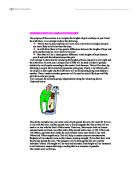
So for example if I estimate a 99% confidence interval of the year 10 boy’s height and when I choose a boy that is in year ten and lives in Leicester there will be a 99% probability that his height will lie between the two values stated. The area under the curve adds up to 1.
90% confident
0 Z1 0.05
0.9
0 = mean (µ)
Ф Z1 = 0.95
So Z1 = 1.645 (from table)
Ф = area to the left
95% confident
0 Z1 0.025
0.95
Ф Z1 = 0.975
So Z1 = 1.96 (from table)
99% confidence
0 Z1 0.005
099
Ф Z1 = 0.995
So Z1 = 2.575 (from table)
To find the confidence intervals you need to know
- standard deviation of the sample
- mean of the sample
- sample size
- standard error
How to calculate the confidence intervals.
µ–Z1 (S.E)> x< µ +Z1 (S.E)
Separate them:
µ< x + Z1 (S.E)
µ> x– Z1 (S.E)
Then put mean in middle stating what it’s more than and less than
……<µ<……
I chose a sample because it is impossible to weigh the whole population. The sample must be random for the Central Limit Theorem to be in effect, so that the distribution of its mean is Normal and predictions can be made about it, even though the distribution of the parent population of heights is unknown and not necessarily Normal.
The population I have chosen for this investigation is the year ten heights in Leicester. I wrote all the names of the schools in Leicester on separate pieces of paper and put them into a hat. I shook the hat and randomly picked one school out. The school that was picked was Beauchamp College. I went to Beauchamp College and measured all the heights of the girls and boys in year 10 and recorded them. I then recorded all the boys’ height and girls’ height on separate spreadsheets. I then used the random button on the calculator to pick 30 boys and 30 girls. When I chose the random number and if the random number was 0.312, I did 3+1+2=6 so I chose the 6th person and as I kept on getting random numbers I kept on going down the list to finally get 30 girls and 30 boys. I did the girls and boys separately. These were the results that were obtained.
These are all my calculations
Summary of results
Mean height of boys = 168.1 cm
Mean height of girls = 160.7 cm
Variance of the boys height = 54.27
Variance of the girls height = 36.36
Unbiased estimator of the population variance of the boy’s height = 56.14
Unbiased estimator of the population variance of the girl’s height = 37.61
Standard deviation of the boys height = 7.37
Standard deviation of the girls height = 6.03
Standard error of the boys height = 1.35
Standard error of the girls height = 1.10
90% confidence interval of the boy’s height = 165.87925<µ<170.32075
90% confidence interval of the girl’s height = 158.89050<µ<162.50950
95% confidence interval of the boy’s height = 165.454<µ<170.746
95% confidence interval of the girl’s height = 158.544<µ<162.856
99% confidence interval of the boy’s height = 164.62375<µ<171.57625
99% confidence interval of the girl’s height = 157.86750<µ<163.53250
Because the variance of the heights is large I cannot estimate the mean of the parent population.
What my results show is that girls don’t grow as tall as boys. What they also show is that boys are not as short as girls. In my sample the smallest girl is 145.0 cm tall and the smallest boy is 154.0 cm tall. In my sample the tallest girl is 171.4 cm and the tallest boy is 184.0 cm.
What this also shows is that the girl’s heights are less varied. They are more squashed together. The boy’s heights are more varied and are more spread out. This can be shown in a stem and leaf diagram.
This investigation could have been better if I took a larger sample size. This would have given me better results. This would have given me a more accurate population variance and more accurate confidence intervals.
To show the spread of the boys and girls height I drawn a stem and leaf diagram.
If I wanted to be 99% that the population mean was ± 0.001cm of the mean of the sample, I would have to take a larger sample.
The z1 score for 99% is 2.575. To obtain the confidence interval (such as the ones calculated above), I would have to multiply this figure and by the s.e. and add it to or subtract it from the sample mean. However, now I have the confidence interval, and I am trying to work out the correct size of the sample so that the standard error is small enough to have a very small confidence interval. In essence I am doing the process backwards.
The size of the sample was small. The calculations that relied upon the data collected are therefore inaccurate to some extent. To be more accurate a large sample must be collected. Accuracy in the realm of to 0.001g is unlikely to be needed, so a larger sample would not necessarily have to be as big as 20,000, which is very impractical
The sample might have been a “fluke” I might have got all the tall girls and boys or all the short ones. However there is not much to do to eliminate the possibility of this apart from to measure every single every boy and girl. This is extremely impractical (possibly impossible).
The children measured were from one area, they do not represent all the children in the world, only ones in that area.