Investigation into factors affecting growth

Introduction

In this project I will be investigating the factors that effect growth such as Male/Female, Age, D.O.B, Height, Foot length, Hand span, Wrist circumference and Pulse. For my population I will be using a sample of data from the “Census at schools project (phase 3)”, which is the most recent. I requested a random sample size of 200 from the “Census at schools project (phase 3)”. The fields of data in the sample are: Male/Female, Age, D.O.B, Height, Foot length, Hand span, Wrist circumference and Pulse. I think that this data is likely to be true and fairly unbiased, even though it is secondary data, I am assuming that nobody except for the person that data applied to has tampered with it, but I can’t be sure. This would make primary, but I have not collected the data myself, therefore I cannot tell if someone is lying or has given a spoof entry. I will be comparing some of the fields; Male/Female, Age, D.O.B, Height, Foot length, Hand span, Wrist circumference and Pulse, to see what links they have with each other, if any. Obviously a sample of 200 is to many for me so I have taken a smaller sample of 51 from the 200. This will be my population. I have chosen 51, because this makes it easy to find the median and the upper and lower quartiles (the 17th, 26th, 34th sample). To choose my population from the larger sample of 200, I used completely random sampling, to do this you use a calculator or computer to generate a completely random number between two points that you select. I have chosen this type of sampling, because in my opinion this is a good way of avoiding bias.

Hypotheses

I am going to investigate and compare 5 of the 8 fields, Age, Height, Foot length, Wrist circumference and Pulse.

Firstly I think that there will be a very strong link between Age and Height, because as people get older they generally get taller.

Secondly I think that there will be a strong correlation between Wrist circumference and pulse, because as people become more overweight they are less fit, therefore having a faster heart rate (pulse).

Thirdly I think that there will be a strong correlation between height and foot length, because as people get taller they will generally have bigger feet. I believe this, because they need more surface area to support there larger bodies, to maintain stability.

I also think that when looking at the pulse of people generally that it will be groped around the lower 2/3rd of the field. This would indicate that most of my sample is quite healthy; this could possibly be as they are young.

These will be the three comparisons that I will be focusing on throughout this project and I will be going over these hypotheses again in the conclusion to see if I can support them or not with my statistical evidence.

Methods of comparing Data

I will be using different ways of analysing the data. Here is a list of all the ways will be comparing the data;

Normal Scatter Graph.

With a normal scatter graphs I can clearly see any correlation and I can apply a trend line if I feel I could put one on the graph.

Grouped Frequency tables.

With grouped frequency graphs, you can get an idea about how skewed the data is, and whether it’s negatively, or positively skewed.

Cumulative Frequency graphs and

Box plots.

These make it easy and more possible to see ...

This is a preview of the whole essay

I will be using different ways of analysing the data. Here is a list of all the ways will be comparing the data;

Normal Scatter Graph.

With a normal scatter graphs I can clearly see any correlation and I can apply a trend line if I feel I could put one on the graph.

Grouped Frequency tables.

With grouped frequency graphs, you can get an idea about how skewed the data is, and whether it’s negatively, or positively skewed.

Cumulative Frequency graphs and

Box plots.

These make it easy and more possible to see the mean and the upper and lower quartiles.

Histograms.

These can give you a good indication of how skewed the graph is and weather the data range is positively or negatively skewed.

The mean, median, mode and range.

This is used to show the average reading of the data; ideally the three M’s (mean, median, mode) will be within a small range of each other giving a more accurate average.

Standard deviation.

Standard deviation is a complex formula that tells you how much the data averagely deviates from the mean.

Spearman’s correlation coefficient.

Spearman’s (rank) correlation coefficient is a great way of being able to measure how much correlation there is between two data sets. It gives you a number between 0 and 1, the higher the number, the more correlation there is.

Analysing data

Scatter graphs

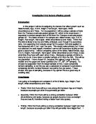
Firstly I will start by producing 3 graphs, these will be of the comparisons in my hypotheses. Fig 1 = Age to height. This has proven my hypothesis completely wrong; there is an extremely weak correlation at the most. This shows that there obviously is very little link between age and height and there are people of the same size 5 years apart, which I didn’t count on.

Fig 2 = height to foot length, on this graph there was a very strong positive correlation, showing that, as people get taller, there feet get bigger. This has proven that my hypothesis is correct.

Fig 3 = wrist circumference to pulse, also in this graph there is another very strong positive correlation. This shows that as the wrist circumference gets bigger the pulse does get higher. This graph has a few outliers, which I did not include, because it would distort the mean point. It is a very strong correlation.

Grouped frequency

In this I’m going to use pulse and I’m going to place them in a group according to their wrist circumference. I’m hoping that I will be able to see of this graph is positively or negatively skewed, or not at all. The wrist circumference range is from 155 - 220cm (a range of 100). I will have four groups with a range of 20cm

By adding together the “Frequency x mid interval value” row and dividing it by the total of the frequency row I can work out the mean.

This grouped frequency table shows me that the mean wrist circumference is 171.7cm. Which is only one centimetre above the mid internal value of the 2nd group. Because of this I predict that the column graph that I produce will be positively skewed.

The graph is positively skewed showing that the people in my data set have a wrist circumference that generally lean towards the bottom 2/3rd’s of the wrist circumference range (Positively skewed) showing that a large majority of the people in my data set are healthy and are not over weight, they could be fit and healthy because they are all under the age of 17 and kids are always healthier than adults.

Cumulative frequency

I have done two cumulative frequency graphs, one on pulse and one on wrist circumference. I used the cumulative frequency graphs to work out the upper and lower quartiles, the median and the range. On the pulse graph, the median was exactly where it is supposed to be on the 70 mark. Which is the average pulse rate for a child aged 11 – 16, I know this from different sources one is the BBC news. Here is a box plot to show the pulse graph.

Key

UQ= Upper quartile

LQ= Lower quartile

M= Median

This box plot shows that the upper quartile 76 and lower quartile 63. This makes the inter quartile range 13, which is not very much, because the field “pulse” has a range of 70, showing that there is a main group just below the middle of the range, and there are a few outliers that are stretching the range out. The lower quartile and upper quartile are almost symmetrical, showing that there is an even amount of rise through the field. Also by using the quartile coefficient of Skewness rule I have discovered that this box plot is negatively skewed.

The wrist Circumference had an even smaller inter quartile range compared to the range of the whole field, the lower quartile is 148 and the upper quartile is 163 and a median of 155 giving a range of 15, in a field that has a range of 180. This range would not be quite so extreme, if it weren’t for an outlier with a wrist circumference of 300, the range would be only 100. But these things have to be counted. This still says that the majority of the field is at the lower end of the range. This box plot is negatively skewed.

Histograms

Using a histogram I will look at the field of “pulse” to see where the majority of data is and identify the modal pulse. This graph shows that the majority of the pulse field is between the 50-80 mark, this shows that the rest of the field is mainly made up of outliers. This also shows that the most common pulse is between 60 and 70 with a mid point of 65. showing that to be the most common pulse.

The Mean, Median, Mode and Range

I will work out the mean, median, mode and range of wrist circumference and pulse.

Pulse

The pulse field ranges from 50-125, which gives a range of 75, which is higher than the average pulse rate for a child aged 11-16.

This picture shows that the range between mode and mean is 9.6, which is a fare-sized range. The mean is 73.6(only 3.6 away from the average), suggesting that the UK is not as fit as it should be, whereas the median is 68.5 and therefore says that the UK is slightly fitter than average. Then the mode is 64, which is way below average, therefore saying that the UK is far fitter than average.

Wrist circumference

The range of the wrist circumference field is 180cm, which would only be 100cm if it weren’t for some outliers. The people who are considered healthy

11-16 year olds according to their pulse rate of 70 have a wrist circumference of 15.5 cm each; I will presume this is the country’s healthy average.

The mean, median and the mode are all within 0.8cm of each other. They are slightly over the healthy average that I predicted, but very close considering that it is a range of 180 and I was only five out this is quite close. It is rare to have the mean, median and mode in such close proximity to each other, so I think that this points towards around 160cm being the average wrist circumference.

Standard Deviation

Standard deviation measures both the variance and how spread the data is from the mean. The bigger the variance, the more spread your readings are.

First I will use standard deviation on pulse and then compare it to the standard deviation of Wrist circumference.

Pulse

Wrist circumference

These two fields have different standard deviations, showing that the wrist circumference field is more spread out, and the readings are not all in won clump much as the pulse field. If you look at the gradient of the pulse cumulative frequency graph, the gradient becomes very steep for a short period of the graph, and then the gradient becomes gentler again. In the wrist circumference graph this happens, but not to the same extent. Most of the people in my sample have a very common pulse rate compared to their wrist circumference, which is more varied across the board, or this could just be because the wrist circumference measurements are to the mm, which is very accurate, whereas the pulse is a lot more vague, because it’s hard to be that specific or accurate with the pulse because it’s measured in time.

Spearman‘s (rank) correlation coefficient

This is a process used to find the correlation coefficient of something if it’s ranked. It is used to show how much correlation there is between two different sets of data, this is a great method of finding this. I have used the computer to find out the correlation coefficient of the two comparisons below and by hand I have found out that the correlation coefficient of age to height is 0.375108082. Showing that there is a very small link between age and height compared to the two comparisons below.

Correlation Coefficient of height to foot length = 0.992223074

Correlation Coefficient of wrist circumference to pulse = 0.849839798

This is probably the best way to prove links between two different fields. And it’s very easy to under stand the number that is produced from it.

Conclusion

From my calculations I can prove some of my hypotheses correct. The higher the pulse, the larger the wrist circumference is a true hypothesis I can prove this from a lot of my calculations especially the normal scatter graphs and the Spearman‘s correlation coefficient. So is the hypothesis that there will be a strong correlation between foot length and height, I have various calculations to prove this, the strongest of which is the Spearman‘s correlation coefficient, because it clearly shows the strength of the correlation. The one prediction that I instantly made, without thinking it through which seemed very obvious at the time, this is; there will be a strong correlation between age and height. All of my calculations prove this to be completely wrong first of all the normal scatter graph; I could barely draw a trend line through it, then the Spearman‘s correlation coefficient was at completely the opposite end of the scale to the other two comparisons, so why was I so instinctively sure that that link would be the strongest. I think it may be because all of your life you have the phrase that “he’s taller because he’s older” drummed into you and then you begin to think that that applies in every situation. The other hypothesis was that most of the people in my sample would have their pulse in the first 2/3rd of the whole range. This was also correct, proven by; various graphs, Histograms standard deviation and especially cumulative frequency graphs, as I have already mentioned the gradient rises very steeply at the start of the graph clearly showing that there is a lot of people in that zone. I think that this project has been very successful in testing my hypotheses as well as finding, which methods statistics calculations work best if you want to work out certain things. I think that if I had used a bigger sample my calculations would be more accurate. Also I think I should have got rid of the major outliers, that were clearly false, at the start, because they dragged my results out a lot. One child said that he had a wrist circumference of 30cm, which is believable, but not that he’s 9 years old and has a 30cm wrist circumference. I think that I managed to use as many methods of statistics analysis that I could have. People could use my investigation to help them investigate the physical aspects of children anywhere around the world, they could take the methods that I think work best and they could use my discoveries. Also people could use the information about the average height and things like that to draw an overall picture of the physique of an average English child.

If I were to extend my investigation further I would g into more detail and I would sample another larger group and deduct the extreme and false outliers.