- In many cases, incorrect information is not recorded, but instead wrong data is provided to give people collecting the information. This is because occasionally, students can be silly or overprotective of personal intelligence and abilities, thus give inaccurate data.
- In some cases, an anomaly is caused by one of the population member being of an odd case that is students who are extremely unintelligent.
The estimates given by pupils of year 10 and year 7 can sometimes vary that different periods of the year and can have a considerable effect on the data
- The estimates given by pupils of year 10 and year 7 can sometimes vary that different periods of the year and can have a considerable effect on the data collected.
- It is also possible that a questionnaire used to acquire the information of all the pupils was not well designed and very difficult to comprehend. It may have included questions that are leading or unclear. This means that some of the students will make errors entering their information. E.g. estimates of the length are taken in ‘mm’ where as the area is taken in ‘cm²’.
Each of these issues may greatly affect the results obtained.
There is positive correlation between the estimates of length A and estimates of length B for year 7 pupils.
The following method of sampling is chosen by me to test this hypothesis.
Random Sample
This is where each member of a population has an equal chance of being chosen. The members to be sampled can be chosen by allocating each of them a number and then by putting all the numbers in a hat and picking out the correct amount .The last 2 digits of random numbers on calculators could also be used.
Advantages : truly random, easy to use , each member equally likely to be selected
Disadvantages : not suitable where the sample size is large.
Now that I have calculated each stratum, I will use random sampling to pick my values. The way I will be doing this is by using my calculator. A random sample is one in which each member of the population is equally likely to be selected. I will press the button RAN# on my calculator after the data range is typed in. This will pick numbers between 0-50, and I will only record the first 30 values given to me. I will record these values in my sampled table.
A bias is anything which may make the data unrepresentative. A bias becomes evident when conclusions are reached which are not based upon facts, but instead because those analysing the data already have certain viewpoints or perspectives.
. When we have to analyse data we need to make sure that our experiment is fair and avoid bias. However, there are a few limitations in using random sampling. The calculator will give me random values, which can affect the overall mean. This is because some of the values do not tell me answers of length A and length B.. These values can be absolute nonsense which will most likely change my mean and affect my scatter graphs.
on how my final graph will look like.
Random Sample For Hypothesis 1
Year 7
I have accepted this hypothesis because I have produced a scatter graph for the above data and there is positive correlation between the estimates of length A and estimates of length B Year 7 pupils.
Hypothesis 2
The distributions of estimates for angle C are similar for both year 7 and year 10.
Methods of presenting data partly depend on the type of data collected. In order to collect my sample for this hypothesis, the following procedure is adopted.
Hypothesis 2
The distributions of estimates for angle C are similar for both year 7 and year 10.
Methods of presenting data partly depend on the type of data collected. In order to collect my sample for this hypothesis, the following procedure is adopted
The type of sampling I will use to choose the numbers of students from each year will be a systematic sample.
. I will use a systematic sample because it is suitable for large sample sizes such as this. I have not chosen random sampling because it is not very appropriate for large sample sizes. I am also using systematic sampling to avoid bias. To do this, I will have to use the nth number from the list provided. This can be done by dividing the total number of values by the strata’s. in this case, it will be 100/50=2.Now I will choose every second number from the data sheet.
table
A visual representation of angle C from sample observations for year 7 and 10 was carried out. The information presented in a table can be more easily grasped if it is presented in a graphical format. There are various graphical means to visualize data e.g. a frequency graph , a frequency polygons etc.
Now that I have collected my sample, I will be making a frequency graph to produce a picture of the data.Although this is available in all statistical softwares in computer, it is simple to perform the calculations by hand. In this case the horizontal scale of the graph will be Angle C and the vertical scale will represent the cumulative frequency. After that I will draw a cumulative frequency curve for each Year .
After making frequency graph and cumulative frequency curve for Year 7 and Year 10 I have to find the median , the upper quartile and the lower quartile and use them to draw box plots for comparison of the two distribution. Box plots provide a useful way of representing the median , upper quartile and the lower quartile of a set of data. They are also useful for comparing two or more distributions.
Graph .
Hypothesis 3
boys are better at estimating Length A than girls.
Methods of presenting data partly depend on the type of data collected. In order to collect my sample for this hypothesis, I have again chosen the systematic sample
Because as mentioned before it is suitable for large sample sizes such as this. I have not chosen random sampling because it is not very appropriate for large sample sizes. I am also using systematic sampling to avoid bias. To do this, I will have to use the nth number from the list provided. This can be done by dividing the total number of values by the strata’s. in this case, it will be 100/50=2.Now I will choose every second number from the data sheet table.
I have to choose a random sample of 50 boys (25 from Year 7 and 25 from Year 10) and 50 girls (25 from Year 7 and 25 from Year 10) through systematic sampling.After sampling I have to find mean and range for boys and girls and compare them.later on shall group the data into suitable class intervals and then I have to find modal class for boys and girls and compare them. The information presented in a table can be more easily grasped if it is presented in a graphical format. There are various graphical means to visualize data e.g. a frequency graph , a frequency polygons etc.
Now that I have collected my sample, I will be making a frequency polygons to produce a picture of the data.Although this is available in all statistical softwares in computer, it is simple to perform the calculations by hand. In this case the horizontal scale of the graph will be Length A and the vertical scale will represent the frequency. After that I will draw a frequency curve for boys and girls to compare them.
There are advantages for frequency polygons in the sense that it shows central tendency and dispersion in the data collected. It estimates, mean, summarise a large data in visual form, shows behaviour and distribution of a variable and can be easily understood due to widespread use in business and media.
There are disadvantages as well linked to it as it fail a visual check of the accuracy, it can easily be manipulated to obtained false impressions. It also requires additional written or verbal explanation
Frequency polygons are useful for comparing distributions. A frequency polygon permits the plotting of more than one distribution on the same set of axes.
The normal curve for boys and girls in my sample is the most common type of frequency polygon. It also describes the same interval variable under different circumstances. A small superimposing of the curve reflects the common relationship between boys and girl’s abilities of estimating Length A.
Graph.
Conclusion
After the Year 10 and Year 7 data sheet provided to me by my teacher, I worked out different samples to carry out different statistical methods by displaying my information on different charts and graphs. I also chose to carry out correlation, and the mean to testify my three hypotheses which I put forward for analysis
Hypothesis 1
Looking at my graph and the lines of best fit that I drew I can see that the Year 7 estimates and Year 10 estimates were positively correlated , so my hypothesis is turned out correct.
Hypothesis 2
By looking at my box plot graphs I would say that my hypothesis is right. Year 7s did not estimate Length A as well as Year 10s did. The inter quartile range of error for Year 10 boys was a lot less than it was for Year 7 boys. This leads me to suggest that Year 7 boy’s estimates were more spread meaning that there were quite a few estimates that were far from the correct answer. Also, Year 7 boys mean of error was closer to zero than the year 7 mean error correct answer than Year 10 boys was and Year 10 Highest and lowest estimates were also closer to the correct answer than Year 7 highest and lowest estimates. This all leads me to suggest that Year 10s performed better in estimating Length A than Year 10s did. These answers also show that once again age may matter because the older you are, the more mathematical terms you have been taught thus year 10s having more experience. It shows that even though the Year 7s were younger than the Year 10, they still could not manage to outperform them. It can also show that Year 10s were more bothered to do this that Year 7 was. Many of the outliers came from Year 7 even though they were a couple from the year 10 sampled values. These outliers probably show that Year 7 were not bothered about what they estimated and put a lot less effort in. The inter quartile range does not differ by too large a margin, and so I believe that there is relatively a fairly high probability that age affects a person’s accuracy at estimating lengths. Therefore, I believe that based on my data, is seems like my hypothesis is false. However, I may be a bit biased saying this as hypothesis 1 proves this statement wrong.
Overall, two hypothesis’ tell me that year 10 are better at estimating but hypothesis 1 may overrule this statement.
Hypothesis 3
By looking at frequency polygon, I would say that my hypothesis is right. The distributions of estimates of Length A for Year 7 are approximately the same as they are for Year 10. The standard deviation also clearly shows that Year 10 estimates were less distributed than Year 7. The standard deviation shows that Year 7 estimate range was 20.419 degrees and Year 10s was 6.892 degrees. This clearly shows that the year 7 standard deviation was much more hence the estimates were much more distributed. Year 7s mean was also a lot closer to the correct answer than Year 10s. Year 7s mean was 32.27 while Year 10s was 26.22. The correct answer was 15 degrees and 26.22 is closest. This shows that age does matter. Year 10 results were generally close to the correct answer and this suggests my hypothesis wrong. This is probably because Year 7 do not have the required skills at year 7 because they year 10 students are more aware of estimation and have a higher range of mathematical skills than year 7.