The length of the next trapezium in figure 1.1 is [f(2) + f(3)](h/2); similarly in algebraic terms [f(α+h) + f(α + 2h)] (h/2).
As a result the total area in figure 1.1 can be given as follows:
[f(α) + f(α+h)](h/2) + [f(α+h) + f(α + 2h)](h/2) + [f(α+2h) + f(α + 3h)](h/2) + [f(α+3h) + f(α + 4h)](h/2) =
[f(α) + 2[f(α+h) + f(α + 2h) + f(α + 3h)] + f(α + 4h)]
Thus the general approximation to for n trapezia is:
Tn= (h/2) [f0 + 2(f1 + f2 + f3 +…+ fn-1) + fn]
where f0 is the first strip and is the last fn strip. Notice that f1, f2, f3 ect. to fn-1 do double duty as right-hand and left-hand body.
Note that is the dependent on the number of trapezia. Thus T16 means that area under the curve is split in 16 rectangles whereas T32 means its split up in 32.
Simpson’s rule is different to the trapezium rule in that it fits a parabola between successive triples of points, whereas the trapezium rule fits a straight line between successive pairs of points. As a result the number of strips must not be even. The formula can be derived analytically and has the advantage of involving the same amount of arithmetic as the trapezium rule with the addition of providing more accurate results. Below is a diagram of incorporating Simpsons rule:
The interval a to b is divided into 2n strips, each of width h. To generalise the formula let f0 be the value at a and let f2n be the value at b. The formula is then generalised to:
Sn= (h/3) [f0 + f2n + 4(f1 + f3 + f5 + … + f2n-1) + 2(f2 + f4 + f6 + …. + f2n-2)]
However, seeing as I am carrying out the mid-point rule then the trapezium rule, I will be using a different version of Simpson’s rule (2Mn + Tn)/3. This is simply due to the fact that it involves less arithmetic than using than using the formula stated in the page above.
The use of polynomials:
The mid-point rule is a second order polynomial which overestimates convex curves. The function I am integrating also follows a convex curve. As a result I expect the consecutive values of the mid-point to decrease as this polynomial overestimates. In addition, being a second order polynomial means that as the number of strips (n) double the absolute error should be multiplied by (1/22). Therefore, I would expect the absolute error of M32 to be (1/22) of the absolute error of M16. This can be represented on a number line with the Mn getting closer to the exact value as n increases. From the number line below, we can see that each gap is a quarter to the one on its right; hence the mid-point rule is an overestimate. In addition this also proves that the mid-point rule is a second order polynomial. However, we should note that the mid-point rule is only an overestimate when the curve is convex. This is also the case for the curve
On the other hand, the trapezium rule is an underestimate and each gap is a quarter to the one on its left. Likewise, the trapezium rule is also a second order polynomial and only underestimates when the curve is convex.
Notice, that the mid-point rule is a mirror image of the trapezium rule and vice versa. This is because the mid-point overestimates whilst the trapezium rule underestimates. Therefore, by using both methods we can confine the exact value between the two different polynomials. This means by obtaining values of Tn and Mn where n is a large number, we can find an accurate approximation to the integral as we know the exact value is between that of Tn and Mn.
Technology:
Most of this coursework will be carried out using Microsoft Excel; an electronic spreadsheet program used for organizing and manipulating data. The program is capable of working accurately up to 16 decimals places; this is also the amount I have chosen to work with in my calculations. Due to its manipulative ability Excel makes the handling of data very easy and saves an enormous amount of time. This is due to the fact that you don’t need to calculate everything; once the formula is entered and two consecutive calculations are complete, the cells can be dragged down and the answers required appear.
Excel is able to do this as it follows the formula and is judicious. The reason I chosen to use a program instead of a calculator is due to its ability to use 16 decimal places whereas a calculator can only give answers accurate to 9 decimal places. In addition, the program will allow me to save time and enable me to print the spreadsheet in a formula and number form; this would not have been possible otherwise.
Finally, the graphs will be drawn using Autograph Version 3.2. This is a mathematical software used for drawing and manipulating graphs. The reason I have chosen to use this software instead of Excel is due to the inability of the latter to provide accurate graphs. Excel finds it extremely difficult to draw complicated curves such as , therefore the use of software is essential.
Error Analysis:
The easiest any to understand and grasp error analysis is by using diagrams; therefore this is the way I shall be explaining it. The mid-point rule (Mn) provides more accurate results as n increases. This was explained earlier in the coursework. The difference between the value of n and n+1 is just 1/22(n). This will be proved below:
By working out consecutive values such as Mn and Mn+1 the results can be compared. In figure 1.3 the area under the
sin (x) can be worked out by multiplying the height (which in this case is 1) by the value of sin (0.5). Therefore the approximation underneath the curve is [1*(sin 0.5)]= 0.479 to 3dp.
Now we can work out the value of Mn+1 (M2), by changing the height to (h/2). In figure 1.4 the approximation to the area underneath the graph is given as
[0.5*(sin 0.25 + sin 0.75)]= 0.465 to 3dp.
Likewise M4 can be worked out as follows; [0.25* (sin 0.125 + sin 0.375 + sin 0.625 + sin 0.875)]= 0.461 to 3dp.
By comparing the values of M1, M2 and M4 the ratio of difference and therefore can be worked put.
M1- M2= 0.014904178 M2-M4 = 0.003624350
The ratio between the differences is (0.003624350/0.014904178)= 0.2421. This means that as the height of the rectangles half (h/2) and the number of rectangles doubles, the error is 1/22. This absolute error can be derived form the following concept:
An area under a curve uses Mn rectangles, each of height h. If the number of rectangles is doubled M2n the height of each is halved (h/2). According to www.enm.bris.ac.uk the absolute error is proportional to h2.
Absolute error ∝ h2 Absolute error = kh2
As a result in the first situation where Mn rectangles are used each of height h, the error is Mn= kh2. However, if the number of rectangles is doubled (M2n) and the height of each is halved (h/2) the absolute error is M2n= k (h/2)2= kh2/ 22. Thus, halving h, or doubling the number of rectangles will reduce the error by a factor of
1/ 22. This is why the mid-point rule is a second order polynomial. Note that this also applies to the trapezium rule; doubling the number of trapezia or halving h will reduce the error by factor of 1/22.
The above theory was vital in my investigation. Finding the value of M524288 under the curve is practically impossible, unless extrapolated estimates are used. This can be explained using table 1.0 below:
* Note that “Mn” indicates an extrapolated estimate
Referring to the use of polynomials on page 4, the gap between M4 and M2 is a quarter that of the gap between M1 and M2. Knowing this simple fact the values of M8, M16, M32 and Mn can be worked out consequently. Table 1.0 is an extract from my spreadsheet and relies on this method of extrapolated values.
The values of M up to M64 are exact values obtained from using the mid-point rule. However, it becomes tedious and time-consuming to carry this any further than M64. In order to work out M128 we have to use extrapolated values. We know that the gap between M128 and M64 is one quarter that of M64 and M32. This can be shown diagrammatically on a number line.
The number line shows that the gap is a quarter to the one on its right. Due to the fact that we know M64 and M32 already, we can work out M128. The value of M128 can thus be extrapolated as [M64 – (1/22*(M32-M64))]. This method of calculating a quarter of the gap between M32 and M64 and subtracting (remember mid-point is an overestimate) from M64 is much quicker than calculating the real value. This is how the values of M above M64 are calculated in my spreadsheet. It must be noted that the assumption being made is that the ratio of gaps (table 1.0) is a quarter, however this is not totally true and an explanation will be given in the interpretation.
Similarly, the trapezium rule is also a second order polynomial and the rules of extrapolated values are also used, in addition to another formula. The new formula is T2n= (Tn+ Mn)/2, it combines both the trapezium rule and the mid-point rule which can be used to save time. The reason this works is due to the mid-point being an overestimate whereas the trapezium rule is an underestimate. For example, if both M8 and T8 are known T16 can be found out by taking their average; this shortens calculations. Likewise, it must be noted that there are errors within the values of Mn above M64 therefore errors creep in the values of Tn. This will also be explained in more detail in the interpretation.
In this coursework I made used the extrapolation method. Table 1.1 is an extract of the spreadsheet I used in this coursework. The values of T up to T128 are worked out using Tn= (h/2) [f0 + 2(f1 + f2 + f3 +…+ fn-1) + fn] whereas those above T128 are worked out using extrapolated values like the mid-point rule. When calculating extrapolated values we are assuming the ratio of gaps is set to continue in the same pattern. This can be explained using a number line.
We know that the gap between T256 and T128 is one quarter that of M128 and M64. This can be shown diagrammatically on a number line.
The number line shows that the gap is a quarter to the one on its left. Due to the fact that we know T128 and T64 already, we can work out T256. The value of T256 can thus be extrapolated as [T128 – (1/22*(T64-T128))]. This method of calculating a quarter of the gap between T64 and T128 and adding (remember trapezium is an underestimate) to T128 is much quicker than calculating the real value. This is how the values of T above T128 are calculated in my spreadsheet. It must be noted that the assumption being made is that the ratio of gaps (table 1.0) is a quarter, however this is not totally true and an explanation will be given in the interpretation.
By looking at the Table 1.0 and 1.1 we can see the ratio of differences. Referring to Lissaman R. (2004), with doubling values of n, the factor by which the absolute error reduces is the same as the ‘ratio of differences’ between successive estimates.
One way of getting around this problem is by using the Simpson’s rule. One particular method of the Simpson’s rule is explained on page 4; however it requires an excess of calculation. As a result I have chosen to use the following version: (2Mn+Tn)/3. The average is twice as close to Mn as it is to Tn. This can be justified by the differences in the errors associated with the two polynomials. This is explained below:
Estimate the area of I=using the trapezium rule and mid-point rule, only using 1 strip.
Trapezium rule: Mid-point Rule:
h= (4-0)/1= 4 h= (4-0)/1= 4
T1 = ½ * 4 * (f(0)+f(4)) = 32 M1= 4* (f(2)) = 16
The area of can be worked out from integration and is exactly 21 1/3. Therefore the absolute error in T1 is (32-21 1/3) = 10 2/3, whereas that in M1 is (21 1/3- 16) = 5 1/3. From this we can see that the absolute error in T1 is twice as much as that in M1.
You can see from inspecting the errors in the trapezium sum and the midpoint sum that the midpoint sum is about twice as accurate as the trapezoidal sum and opposite in sign. This explains the weighting of the formula (2Mn+Tn)/3. By using the Simpson’s rule we will have cancellations of the errors and should thus get a much more accurate approximation.
The advantage of using the Simpson’s rule is that it’s a fourth- order polynomial. As mentioned before Simpson’s fits a parabola between successive triples of pairs. The absolute error is proportional to h4 so it is able to achieve a more accurate approximation to the curve,.
Absolute error ∝ h4 Absolute error = kh4
As a result the absolute error is Sn= kh4 whereas the absolute error in S2n= k(h/2)4. This means the errors reduces by a scale factor of 1/16 between each successive Sn values. In theory, the results I have obtained for Sn should be more accurate and reach the exact value in fewer calculations. This is seen to be the case by looking at the spreadsheet attached to this coursework.