Numerical solution of equations
Pure Mathematic 2 Coursework
Numerical solution of equations
By Michael Pang
I am going to show 3 of the numerical methods for solving the equation which cannot be solved algebraically. They are interval estimation, fixed point estimation and Newton-Raphson method. Those of these numerical methods are used when algebraic ones are not available.
When you found any equations which cannot be solved algebraically, probably you will draw the graph and see where the roots are. However, the other problem is found that you cannot get all roots accuracy. Actually, the numerical methods cannot find the exactly root but the answers are more accuracy than sketching the graphs. Therefore, we usually provide the answer to 5 or 6 decimal places depending on what the questioner needs. Finally, we check the answer by setting the lower bound and upper bound to see whether it has sign change or not.
Even if the three numerical can solve the equation non-algebraically, they have its advantages and disadvantages. And now I am going to show how these methods works and their problems by using the equation F(x) = x³-9x+3.
Interval estimation
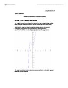
Assume that the roots of the equation F(x) = x³-9x+3, and I am looking for the roots which F(x) = 0.
The roots of the equation are the values of x which the graph of y = x³-9x+3 crosses the x axis. By using the computer, I recognise that there are 3 roots on the graph and the value of these 3 roots. However, if we cannot use the computer, we have to use one of the numerical methods - interval estimation. A root must be lying on the interval a and b where an interval have been marked in which F(x) change signs. We thus know that there must be a root in that interval. The equation F(x) = x³-9x+3 has 3 roots which are in the interval of (-3,-4), (0,1) and (2,3). We can find the roots through decimal search, interval bisection and linear interpolation.
Decimal search
It is one of the methods of interval estimation through dividing each interval into 10 parts and looking the sign change. Here are three steps of this method:
- Take increment in x of size 0.1 within the interval of the root. Stop when there is a sign change.
- The interval has been narrowed down and now keeps on taking increment in x of size 0.01 within the narrowed interval. Stop again if there is a sign change.
- Repeat the step by taking increment in x of size smaller up to 6 decimal places (the final answers are recorded to 5 decimal places.
In the diagram (Appendix A), I have followed all the steps and finally found all the roots. They are 2.81691, 0.33761 and -3.15452 which are the same as the result from the graph.
The only advantage of this method is that the upper bound and lower are found automatically. However, the procedure is long and bored. Therefore, mistakes are easily made if you didn't check it. In addition, without the help of computer, it wastes much time to record every number you have found.
Interval bisection
It is very similar to the decimal search. It has to look at the sign change and divides the interval. However, the interval is bisected and narrowed down the interval depends on how the sign change (negative or positive). Here are the following steps:
- Find the interval which the root is between it and start by taking the mid-point of the interval. For example, the interval between the biggest roots is (1,0), I have chosen it since there is a sign change. And the mid-point of the interval 0.5.
- Put the ...
This is a preview of the whole essay
Interval bisection
It is very similar to the decimal search. It has to look at the sign change and divides the interval. However, the interval is bisected and narrowed down the interval depends on how the sign change (negative or positive). Here are the following steps:
- Find the interval which the root is between it and start by taking the mid-point of the interval. For example, the interval between the biggest roots is (1,0), I have chosen it since there is a sign change. And the mid-point of the interval 0.5.
- Put the mid-point into the equation and find the value of x where F(0.5) = -1.375. F(0.5)<0, since F(0)>0, therefore the root is in the interval (0.5,0). Now take the mid-point of the next interval which is 0.25.
- Put the found mid-point into the equation and find the value of x. The root will be narrowed closer and closer. Stop until you find the value of x is up to 5 decimal.
In the diagram (Appendix B), the same roots are found which are 2.81691, 0.33761 and -3.15452.
This method is slow and boring. Either do it by computer or manually, mistakes are also be made. The only advantage is the same with decimal search, which upper bound and lower bound are found automatically.
Linear interpolation
This method not only use of the sign change of the end point of the interval, but also use of its values to narrow the interval. Chord is also used as finding the x co-ordinate of the point where it crosses the x-axis each time. Here are the steps showing the work:
- Choose the interval where there is a sign change. For example, I chose the biggest root this time and the interval is (2,3).
- Find the value of F(2) and F(3) where F(2) = -7 and F(3) = 3. Chord is then used as joining the curve between (2,-7) and (3,3). To find the x co-ordinate in detail, it is necessary to find the equation of the chord first. It was found as y = -10x + 27, put y = o and then x is 2.7. Put 2.7 into F(x) which F(2.7) = -1.617.
- The interval is then found between (2.7,3) since F(2) < 0 and F(3) > 0. Chord is then used as joining the curve between (2.7.-1.617) and (3,3).
- Repeats the all above steps until the root is found up to 5 decimal which is not changed. The interval change can be occurred on both sign.
Again, in the diagram (Appendix C), the answers have been found as 2.81691, 0.33761 and -3.15452.
After a few times of researching, the decimal place of x is getting larger and larger. Even if I can look for x value which the chord crosses by searching the graph, the value is not accuracy. In addition, when I was finding the equation, it is very easy to make mistakes since there are too many decimal place of value x. Unless I am very good at computing, otherwise it is hard to use simple equation in excel to find the answer at the standard of AL. Moreover, I have to check the upper bound and the lower bound to make sure the root is right. One more problem is the rate of convergence can be so variable. In my case, I have taken the least 6 steps for my middle answer. But I have taken 11 steps for my smallest root. This method should be used the least because the procedures are the most complicated and take the longest times.
Advantage of the interval estimation
In interval estimation, it is not difficult to find the upper bound and lower bound and the end of working. In decimal search and interval bisection, I don't have to check the answer by finding the upper bound and lower bound as the sign change have been showed in the process.
Disadvantage of the interval estimation
Those methods of interval estimation not only waste time and complicated, but also there are several problems which usually found in other equation. They are
- The curve touches the x-axis
- The roots are close together
- There is a discontinuity
The curve touches the x-axis
In the above graph, the curve touches the x-axis. Therefore, the sign change could not be found and none of the methods of interval estimation can be used.
The roots are close together
In the graph, there 3 roots close to together between the interval (0,1). In decimal search, F(0.1) = 0, so that 1 of the root is 0.1 and so further interval cannot be found. In addition, interval bisection and linear interpolation would be unaware of the existence of other roots since the 3 roots are too close together.
There is a discontinuity in F(x)
This equation y = 1/(x-1.1) has no root, but all change of sign methods will converge on a false root at x = 1.1
Avoid problem
To avoid those problems occurring, it is important to start by sketching the graph and therefore the problem will be found.
Fixed point estimation
It is much different from the method of interval bisection. It involves an iterative process rather than finding interval within the roots must lie. Generally, iterative process means that a sequence of numbers by continued repetition of the same procedure. But this method has some limited which will be introduced when the process are showing.
How does it method work?
Before starting to use this method, the equation F(x) = 0 has to be rearranged into the form of x = g(x). For example, in the above graph y = F(x) = x²-3x-4. To rearrange into the form of x = g(x), the equation are then changed to y= g(x) = (x²-4)/3, thus equation y = x is form.
Form the diagram, it is not difficult find that any values of x for which x = g(x) is clearly a root of the original equation by finding the points of intersection of the curve y = g(x) and the line y = x.
Now I am going to use this method to find the roots of my equation X³-9x+3.
The choice of g(x)
The convergence of the x = g(x) allows a root a of the equation, provided that -1 < g'(a) < 1 for the values of x close to the root. A rearrangement cannot converge all the roots, so the other rearrangements of F(x) into the form of x = g(x) are needed.
Now I rearrange the equation in one of the way:
X³-9x+3 = 0
x = (x³+3)/9
x = g(x) = (x³+3)/9
y = x
y = g(x) = (x³+3)/9
In this case, g(x) = (x³+3)/9, it only converges the root in the interval (0,1) since its gradient is between the range of -1 and 1. The gradient is showed below:
Put x = 2.5, g'(a) > 1
Put x = -3, g'(a) > -1
Put x either = 0 or 1, -1 < g'(a) < 1
Therefore, we know that g(x) = X³-9x+3 = 0 only converges the root in the interval (0,1).
After find out where the root(s) is converged, I am going to show the steps to find how the root will be found.
- Choose the value, x1 of x, which is -1 < g'(1) < 1.
- Find the corresponding value of g(x1)
- Take the value of g(x1) as the new value of x, where g(x1) = x2
- Find the value of g(x2) and so on.
The steps are showed on the graph below and the procedures are showed in the Fig.2a in Appendix D. This type of diagram is called staircase diagram.
Find the other root
As I have mentioned before, one rearrangement of the equation is not enough to find the all roots since it cannot converge all the roots. Therefore, I rearrange it into other form of g(x):
X³-9x+3 = 0
X = ³V (9x-3)
X = g(x) = ³V (9x-3)
Y = x
Y = g(x) = ³V (9x-3)
In this case, g(x) = ³V (9x-3), it only converges the root in the interval (2,3) and (-2,-4) since their gradients are between -1 and 1. However, it doesn't converge the interval (0,1) because this time its gradient is larger not the range of -1 and 1. Their gradients are showed below:
Put x = 2, -1 < g'(a) < 1
Put x = -2, -1 < g'(a) < 1
Put x either = 0 or 0.5, g'(a) > 1
Therefore, the equation doesn't converge the root in the interval (0,0.5). The others 2 roots will be found which are showed on the graph below and its procedures are showed in the Fig.2b and Fig.2c in Appendix D.
Upper bound and lower bound
To ensure the roots are right, establishing bounds for the root are necessary as this method doesn't show the upper bound and lower bound automatically. They are showed below:
- The largest root : F(2.816915) = 0.0000142, F(2.816905) = -0.00013403
- The medium root : F(0.337615) = -0.00005233 F(0.337605) = 0.00003425
- The smallest root : F(-3.154525) = -0.00004153 F(-3.154515) = 0.00016701
It proved that I didn't make any mistakes about finding the roots because there is a sign change between the upper bound and the lower bound.
Advantages
Compare with the method of interval estimation, the processes are easier to find and faster. Even if do it without the help of computer, the mistakes are not easy to make. So I didn't feel cumbersome.
Disadvantages
During the processes, 2 rearrangements have to be rewritten into the form of x = g(x). It's not difficult but if I sketch the graph without computer, the process is quite boring and difficult to sketch by written. Moreover, additional information such as gradient function has to find as well, in order to check whether the root is converged by g(x) or not. In addition, upper bound and lower bound are not found automatically, so I have to find it myself to check if the root is right or not.
The Newton-Raphson method
Actually it is another fixed point method, it has to find a starting point by estimating and draw the tangent to the curve y = F(x) at the starting point. Now I am going to show how Newton -Raphson was come out.
- Draw a tangent at x1
- X2 is the intercept of tangent with the x-axis
- can be written as as y = F(x), m = F'(x)
- At the point of x2, y2 = 0, therefore, the equation can then be changed to
- Then the equation will then be changed to
- Finally, Newton - Raphson method is finally written as
The processes
In my case, F(x) = x³-9x+3, each root, from large to small, I have chosen their value of x1 are 3, 0 and -3. And F'(x) has been found as 3x²-9. Therefore, I got enough information to find the root and I follow the steps I have showed the page before and the procedures are showed on the appendix E.
Refer to the appendix E, the roots are 2.81691, 0.33761 and -3.15452 which are same as I search in the graph. The other methods to show they are right, I should check their upper bound and lower bound where I set it in Fixed point estimation. And now I show it again to make it clear.
- The largest root : F(2.816915) = 0.0000142, F(2.816905) = -0.00013403
- The medium root : F(0.337615) = -0.00005233 F(0.337605) = 0.00003425
- The smallest root : F(-3.154525) = -0.00004153 F(-3.154515) = 0.00016701
Advantage
Newton-Raphson method is fast and convenient, the processes are short and that why I didn't use a lot of presentation to show my understanding. It also gives an extremely rapid rate of convergence. I only use 4 to 5 steps for each of the root, so I find that it was much easier to finish than the first 2 methods.
Disadvantage
Even this method is the fastest and the most convenient, it still has several problems.
Firstly, in my case, if I didn't choose the right initial value, I couldn't find the root by only 4 to 5 steps or even faster in other case. However, if the first value I h chose is not close to the root, or near the turning point, a turning point of y = F(x), the iteration may diverge, or converge to another root. And if the initial point is at a stationary point, F'(X) = 0 so the method cannot proceed.
Secondly, all numerical methods for solving equations cannot be proceeded when the function is discontinuous function as it doesn't have any real roots.
Thirdly, the function is not defined over the whole of. The tangent at the graph may meet the axis at a point outside the domain of the function.