Differentiate the equation f’(x) = 3x²-13.
x2= 3 – 3³- (13*3)+14
(3*3²)-13
x2= 3 - 2
14
x2= 2.85714
By using this same method, but shortened significantly by using the ANS button on my calculator, I will find x3,, x4 etc
x3 = 2.84423
x4 = 2.84181
x5 = 2.84134
x6 = 2.84125
x7 = 2.84123
x8 = 2.84122
x9 = 2.84122
The graph shows the process
The root is 2.84122 to 5 significant figures ( + or - 0.00005) as there has been repetition to this level of significance
To check this is the root to this error bound, I will check the sign of the y-co-ordinate on each side of the root. It should be different on each side if the line crosses the x-axis.
f(2.841225) = 0.0000329 Positive
. f(2.841215) = -0.0000793 Negative
There is a change of sign so there is a root there to this significance. I am now going to find the other roots.
x1 = 1.07692
x2 = 1.20810
x3 = 1.21482
x4 = 1.21484
x5 = 1.21484
So, for the last root I will try x1 as –3.
x1 = -3
x2 = -4.85714
x3 = -4.20901
x4 = -4.06333
x5 = -4.05608
x6 = -4.05606
x7 = -4.05606
f(-4.056065) = -0.000171 Negative
f(-4.056055) = 0.000193 Positive
Failure of Newton Raphson method
The method fails if the initial value is not close to the root, or is near a turning point of y = f(x), the iteration may diverge, or converge to another root.
Equation : x5 + 2.1x4 + 0.8x3 + 0.7x2 – 0.4x – 0.9 = 0
For the starting value of
x0 = 0 and therefore to find the root between x = -1 and x = 0
Differentiate dy =5x4 + 8.4x3 + 2.4x2 – 1.4x – 0.4.if x0 = 0, dy/dx = -0.4.
dx
The gradient of the tangent is negative. And as shown in the graph, the Newton – Raphson method converges to the root close to x = -2.
Rearranging Method
In this method the equation f(x) = 0 is re-arranged in the form x = g(x).Using the formula f(x) =0 another formula g(x) = x is derived, and the root can be found of the equation.
Re-arranging the formula to get the equation in the form of x = g(x). One of the many different forms of the equation is y = x5-3x+1
y = x5-3x+1 shows the roots lie in the intervals [-2,-1], [0,1] and [1,2].
x5-3x+1 = 0, therefore x = x5+1
3
We get the formula: xn+1 = xn5+1
3
The curves above show y = x and y = g(x) = x5+1.
3
I am going to find the root between [0,1]. I will take 1 as my starting point.
The iteration has found the root to an accuracy of 5 significant figures when x = 0.33473 (x = 0.334730 ±0.00005). This can be shown by replacing the lower and upper error bounds into y = x5-3x+1.
When x = (0.334735 +0.00005) = 0.334735, y = -2.52 x 10⁻⁶ (y is negative).
When x = (0.334735 - 0.00005) = 0.334725, y = 2.69 x 10⁻⁵ (y is positive).
Failure of Rearrangement Method
This method fails whenever the line diverges. As you can see the root in the interval [0,1] was correctly found as the gradient of g(x) falls within the acceptable boundaries. However, one iterative formula is not always successful at finding the other roots of an equation.
When x = 2, the iterative formula actually diverges away from the required root in the interval [1,2]
As you can see, the iterations just keep getting further and further from the point. It’s because the formula involves squaring the last number, so will never staying low for long.
Comparison of method
I am now going to make a comparison the three numerical methods that I have used. For fixed point iteration I tried to find a root of y = x5-3x+1. I will now try to find one root of y = x5-3x+1 using decimal search and Newton-Raphson and I will then compare the relative merits of the three methods in terms of speed. I will also talk about the advantages of computer software when using these three numerical methods.
Fixed point iteration: Earlier on it took six calculations to find one of the roots of f(x) = x5-3x+1 to be equal to x = 0.33473 as well as the initial step of rearranging y = f(x) into the form x = g(x).
Decimal search: I will now attempt to find the root of y = x5-3x+1 in the interval [0,1] using decimal search, to an accuracy of five decimal places
It took me 5 steps to find
the change of sign in y.
It has taken another
five steps to find the root to
an accuracy of 1 decimal place.
I am continuing this process of decimal search
until I find the required root to an accuracy of five decimal places
It has taken me thirty-six calculations to find the root to an accuracy of five decimal places (x = 0.33473 ±0.000005).
Newton-Raphson
I am going to find the root of y = x5-3x+1 in the interval [0,1].
xn+1 = xn – f(xn)
f’(xn)
Differentiate f’(x) = 5x4 - 3
It only took three steps to confirm that x = 0.33473 ±0.000005
Which method is Quickest?
From the 3 results shown above, I can clearly conclude that the Newton-Raphson method is the quickest one, because it gives the fastest convergence. It does reply on being able to differentiate the f(x) though.
The Decimal Search method is quite a slow method, because it takes a lot of time to prepare the spreadsheet on Excel: especially the various formulas for the different calculations. And as shown above it takes many iterations to find the root. But it will only take a few minutes for someone who knew how to use the software to find the root to the required degree of accuracy.
Newton-Raphson was the quickest of the three numerical methods. Newton-Raphson took only four steps and fixed point iteration took six steps to converge to the required root. The use of Microsoft Excel did not make a huge difference because a scientific calculator can easily be programmed with the required iterative formulae. A few presses of the ‘equals’ button would converge to the required root.
The most likely problem with Newton-Raphson was finding the wrong root if the tangent diverges away from the required root. Decimal search also had a problem by not showing a change of sign in the first set of calculations when the root had two decimal places.
The Rearrangement method takes a lot of time to find the right arrangement of an equation, because not all g(x) graphs will allow convergence to the required root. Graphamatica was a very useful piece of software as it could be used to instantly visualise curves and gradient functions. This meant that within seconds I could produce an accurate curve instead of having to make some calculations and draw the curve myself. This saved a lot of time as I could easily pick appropriate starting values without having to waste time using trial and error to pick my starting value.