The iteration converges to the root xn = x4, relatively faster than the other methods have seemed to.
The root within the interval [1,2] can be written as:
- 1.175 with a maximum error of ± 0.005, or
- 1.2 (to 1 d.p.).
To find the root graphically, we must first make an estimation where the root is along the x-axis (x1), and draw the tangent at the point where x = x1 touches the curve. The point where the tangent cuts the x-axis gives us the next approximate value for the root, and so the process is repeated until convergence is noted. Using the previous equation and root interval to prove the root graphically, starting with the same x1 value (x1 = 1.5.)
Drawing the initial tangent to the curve gives us a second approximate x2 = 1.336.
Further tangents provide us with the xn values:
x |delta x|
x2 1.336 0.1639
x3 1.23 0.106
x4 1.182 0.04829
x5 1.172 0.009886
x6 1.172 0.0003846
x7 1.172 5.702E-07
x8 1.172 5.72E-12
x9 1.172 0
From this close – up of the final tangent drawn we can see that the root within the interval [1,2] is 1.172 with a maximum error of ± 0.005.
Newton – Raphson Method Failure.
There are three main problems that appear with the Newton – Raphson method –
- Bad choice of starting value – when x1 is close enough to the root, the method will nearly always converge towards it, but if x1 is either near a turning point of y = f(x) or too far away from the root, the iteration may either diverge or converge to another root.
A way to see if the initial approximation for x1 is close to a turning point is to see the size of f’(x) – if it is small, this will cause the value of x2 to be far away from the root in most cases. This may cause rapid convergence to another root of the equation after two or three steps. Also, when x1 is a stationary point (therefore f’(x1) = 0) the method cannot proceed.
- The function is discontinuous – this is the same with all numerical functions.
- The function is not defined over the whole of real numbers – this will cause the tangent at (xi, f(xi)) to meet the axis at a point outside the functions domain.
An example of a Newton – Raphson method failure – using the equation
y = x^3 – x^2 – 8x +11.
For this I shall be using the graphical method of Newton – Raphson iteration. The initial graph of y = x^3 – x^2 – 8x +11 is:
This shows that the equation has roots within the intervals [-3,-2], [1,2] and [2,3]. I shall try to find the root within the interval [1,2], taking x1 = 2.00.
From this we can see that when a tangent is drawn from the initial approximation, it touches a stationary point when it reaches the curve, and so draws a horizontal line. This horizontal line (equation y = -1) will never touch the x – axis, and so cannot provide us with an approximate x2 value, and so the method fails.
This is an example of a bad choice of starting value – as the starting x value chosen made a tangent with a stationary point, and so the line drawn will not go back to the x-axis, but only run parallel to it.
Fixed Point Iteration – Rearranging f(x) = 0 into the form x = g(x).
Initially, the equation f(x) = 0 must be rearranged into the form x = g(x). any value of x for which x = g(x) shows to be a root of the original equation.
Using the function f(x) = x^5 - 4x – 2 gives the graph:
From this we can see that there are three roots, within the intervals [-2,-1],[-1,0] and [1,2].
-
one rearrangement: x = g(x) = x^5 - 2 which gives us the graph:
4
Taking x = 2.0 as the starting point to find the root within the interval [-1,0] – we gain the following set of results:
This rearrangement provides the basis for the iterative formula:
Xn+1 = x^5n - 2
4
This gives the set of results:
This shows the root to be –0.50850 within the interval [-1,0], which can be written:
- -0.509 with a maximum error of ±0.0005, or
- -0.5 (to 1 d.p.)
Displayed graphically:
From which we gain the root as –0.5085 (to 4 s.f.) from the results box, which again gives the root in both the ways written above.
As f(x) = x^5 – 4x – 2
And g(x) = x = (x^5 – 2)/4
The magnitude of g(x) for the results gained above can be shown to be:
This shows that the magnitude is always less than one, and as the method will only succeed if -1 < g’(x) < 1 , and as this is the case for all the values of x found, the method works.
Method Failure
We can see that this rearrangement of f(x) works when trying to find the root within the interval [-1,0], but I shall now try to find the root within the interval [1,2] using the same method.
Taking the starting point as x1 = 1.8 gives the following table of results:
We can see from this that the x value is getting increasingly larger, which can be seen on the graph as:
We can see from this that the method has not converged to the root, and by looking at the magnitude of g’(x) for these values of x:
We can see that the magnitude of g’(x) is increasing far above 1 for each x value, and so the condition -1 < g’(x) < 1 is not fulfilled, therefore the method fails.
This shows that the method can sometimes be used on a single rearrangement to find one root, but not necessarily another. The condition -1 < g’(x) < 1 must be fulfilled in order to gain convergence to the root, and so shows that (x^5 – 2)/4 is a suitable iterative formula for finding the root within the interval [-1,0] but an unsuitable iterative formula for finding the root within the interval [1,2]. To find this root, either another method would need to be applied or a different rearrangement found that is suitable for finding this root.
Method Failure
There are several ways that the change of sign method can fail:
- There are several roots close together.
This can make it easier to miss one of the roots when there are several within a small interval, because when using the manual change of sign methods, one root would be found and generally more would not be looked for. Without the aid of a graph you would not know that you had missed one or maybe more roots.
- The function f(x) is discontinuous.
Discontinuities such as asymptotes provide problems with the change of sign method as they cause convergence at a false root, and again – without the aid of a graph or knowledge of the curve would cause an incorrect root to be found.
- The curve touches the x – axis.
If the curve simply touches the x-axis but does not actually cross it, then there will be no change of sign, and so the change of sign methods have no chance of being able to work.
Example:
If we zoom in on this possible root, we can see that it touches the x – axis within the interval [1.6,1.7].
If a decimal search is performed within this interval, using increments of size 0.01:
We can see from this that the curve touches the x – axis when x = 1.67, but as the curve does not actually cross the line, there is no change of sign and so the method fails.
This is an example of the third type of method failure, where the curve touches the x – axis but does not actually cross it.
Comparison of Methods.
I will be using the equation x^5 – 5x + 3 = 0 in order to compare each of these numerical methods. This is the equation used to investigate the change of sign (decimal search and interval bisection) method. The graph of f(x) = x^5 - 5x +3 is:
Rearrangement of f(x) = 0 into x = g(x):
One rearrangement of f(x) = 0 into the form x = g(x) could be:
x = g(x) = (x^5 + 3)/5
The iterative procedure of this rearrangement shows to be:
xn+1 = (xn^5 +3)/5
Looking for the root within the interval [0,1], with x1 = 1, gives us the calculation results:
Here we can see that the iteration has converged quite rapidly to the root within the interval [0,1], giving us a root of 0.6180 with a maximum error of ± 0.0005.
To find this root graphically, we need to draw the graph of y = g(x) and y = x on the same axis, which gives us:
Showing this graphically, we need to take the starting point on the x-axis, which I will take as x = 1 as I am trying to find the root within the interval [0,1]. Adding this in the ‘Parameters’ box of our graph program, and with continued iteration until the root is found gives us a graph that shows:
This shows a ‘staircase’ converging on the root within the interval [0,1], and from the ‘Values’ box we gain the value of x = 0.618 (to 3 s.f.) when n = 22. This method works as the magnitude of g’(x) = 5x^4/25 in the vicinity of the root within the interval is less than 1:
This can be shown by the following table of results:
The root can be written:
- 0.618 with a maximum error of ±0.0005, or
- 0.6 (to 1 d.p.),
which is the same result gained with the Change of Sign – Decimal Search method.
Newton – Raphson Method.
Again I am trying to find the root within the interval [0,1] – and so using x = 0.95 as my starting point for x, because a starting point gives us a horizontal tangent which would cause the method to fail as it will never cross the x – axis. The initial tangent appears as:
Continuing with this procedure gives the following convergence:
This shows to be about a point within the upper end of the interval [0.61,0.62], which is shown to be 0.618 (to 3 s.f.) and is reached when n = 8. Again, this can be written as:
- 0.618 with a maximum error of ± 0.0005, or
- 0.6 (to 1 d.p.).
This is the same root gained within the interval [0,1] for the change of sign and rearrangement methods, but with the Newton – Raphson method, the speed of convergence is far greater than with the previous two methods.
All of these methods have their problems that will cause them to fail, which have been explained within each individual section. However, with the merits for each that have been discovered during this investigation, the disadvantages of each method begin to alter in significance according to the strength of these advantages.
Both the change of sign and Newton – Raphson methods will fail if there is a discontinuity in f(x), but the change of sign decimal search method is far more laborious and cannot be solved simply by using the graph if being done ‘manually’ – the speed of convergence is far slower than both the other methods, coupled with the ease of method failure and the time taken to perform it is relatively the ‘weakest’ of all the methods investigated.
The two fixed-point iteration methods – the rearrangement of f(x) = 0 into the form x = g(x) and the Newton-Raphson methods have the fastest rates of convergence – but as shown in the comparison above, the Newton-Raphson method is by far the fastest of all the methods investigated. It is also quite hard for the method to fail when the function is continuous, as long as the function is defined over the whole of the real numbers and a suitable starting point is chosen – this may require some testing though, as a difference of 0.05 can mean convergence on the correct root, convergence on the wrong root or failure of the method. Rearrangement of the formula may have a faster convergence than the decimal search method and be far less lengthy, but it is the most prone to failure. Using one rearrangement of a function may cause the method to find all the roots correctly, while a second rearrangement of the same function may cause the magnitude of g’(x) to be greater than one and so the method will fail.
The hardware and software that have been used in this investigation are a scientific calculator and a graph drawing program – Autograph. This allows us to find the roots of each graph without having to draw each of them out along with the tangents, and gives as accurate results for the roots with our own specification on the number of significant figures. This program proves little use for the decimal search method, other than establishing the intervals the roots lie in – the main body of work must then be done through calculations and recording of results, and each significant figure must be found one at a time.
The fixed-point iteration methods benefit greatly from the graph program, as they allow us to gain all the tangents and converging ‘staircases’ and ‘cobwebs’ simply by typing in the starting value of x. This gives us much faster convergence than calculating, and a graphical representation of what is happening, so that we can more fully understand the way each method works. Both are simple to use as long as the equation and the starting point for each interval are known.