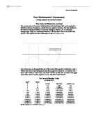
The graph does not clearly show the number of roots on the interval 0 and 1.
The Interval Bisection Table
x³-1.8x²+x-0.17=0
The method is applied successfully to find one of the roots of the equation
x³-1.8x²+x-0.17=0. But the graph drawn to a suitable scale immediately shows that there is more than one root on the same interval.
Applying the interval bisection method would lead to a loss of the other two roots.
This method fails to find the other two roots between 0 and 1.
Newton-Raphson method
In this method it is necessary to use an estimate of the root as a starting point. So starting with an estimate,, for a root of f(x)=0. Then drawing the tangent to the curve y=f(x) at the point (, f()). The point at which the tangent cuts the x axis then gives the next approximation for the root and the process is repeated.
The equation I took for this method is x³-7x+1=0.
It looks like this:
The gradient of the tangent at (, f()) is f ‘(). The equation of the straight line can be written as
y-=m(x-),
the equation of the tangent is:
y-f()=f ‘()[x-].
This tangent cuts the x axis at (, 0), so:
0 -f()=f ‘()[-].
Rearranging this gives:
=-.
=> the Newton-Raphson iterative formula:
As my equation is x³-7x+1=0, with the root in the interval [2, 3], I can rewrite it as:
f(x)= x³-7x+1=0 and f ‘(x)=.
The iterative formula is therefore:
=
Starting with the point =3 gives
The Newton-Raphson method gives an extremely rapid rate of convergence.
The first root of the equation I found is 2.571201 with the error bounds of 2.571200<x<2.571202.
The other two roots can be found using the same table and starting with the value 1
and the value -2.
The method is applied successfully to find all three roots of the equation.
Problems:
Almost all the problems that may arise in this method fall into one of the possible categories such as
Poor choice of starting value:
If your initial root is close enough to a root, the method will nearly always give convergence to it. However if the initial value is not close to the root, or is near a turning point of y=f(x), the iteration may diverge, or converge to another root.
For example the equation of
In this case the iteration diverges and is unable to find the root.
Fixed Point Iteration
In fixed point method a single value or point is estimated for the values of x, rather than establishing an interval within which it must lie. This involves an iteration process, a method of generating a sequence of numbers by continued repetition of the same procedure. If the number obtained in this manner approach some limiting value, then they are said to converge to this value. The first step, with an equation f(x)=0, is to rearrange it into form x=g(x). Any value of x for which x=g(x) is clearly a root of the original equation.
For the next method I decided to take this equation:
The first step is to rearrange the equation into the form of x=g(x). Any value of x for which x=g(x) is clearly a root of the original equation.
The graph shows the equation and y=x.
The equation can be rewritten in a number of ways, one of these is
x=g(x)=
And this creates an iterative equation:
Taking x=-1 as a starting point to find the root in the interval [-2, -1], successive approximations are:
In this case the iteration has converged quite rapidly to the root I was looking for.
There is a problem when this method cannot be applied. This can occur when the gradient is greater then one. In that case you got the overflow and can’t estimate the root.
For example the same rearrangement may fail if you try to find the other root.
It would diverge and cause the overflow.
Comparison of methods
For this part of my coursework I’ve chosen the following equation: x³+2x²-x-3=0.
As I used the same equation as in the first method of my coursework then I can get the result from the table above, which is
1.14794921 to (5 d. p.)
with the possible error value of 0.00048828125.
Newton Raphson method:
Using this method I found the estimation of the root to be 1.148 with max. error 0.00057. So the next method is change of sign. From the graph I decided to estimate the root to be between 1 and 2.
So after building the table we can see that the root is estimated to be 1.147949219 with possible error of 0.0004883.
Fixed point iteration:
Getting the result of 1.1479 to 4 d.p.
So after estimating the root using several methods I can say that the most exact result with the smallest maximum error level can be obtained using the change of sign method. The advantage for this method is that it is reasonably safe and every estimate of the root is accompanied by solution bounds, namely the end points of the smallest interval in which you now the root lies.
But despite of this it takes lots of time to obtain one root and would take ages to do it without any computer or graphic calculator aid. Also the initial search may miss one or more root, for example when the x-axis is a tangent to the urve or when several roots are very close together.
Newton Raphson method is the easiest way to estimate the root and takes much less time than to estimate the root using the first method. It doesn’t take that much time but it can go wrong very quickly and jump to another root.
And the last method rearranging is the hardest one. It takes plenty of time to rearrange the equation and then to estimate the root. And it’s very likely to do something wrong using it.
In conclusion I can say that the most efficient and easiest way for me to estimate the root, was the first one, because it takes not so much time if you get used to it. Very useful were PC programs such as Excel and Autograph. And at last the fact that in excel it is easier to change one equation on another and to get other roots, I can definitely say that it is the best method for me.