So, using these tables we can say that the root is 1.17740965 with maximum error bounds of ±0.00000005. I think this is accurate enough.
Advantages and Problems with the Change of Sign Method
There are of course advantages and disadvantages of this method of solving equations.
The main advantage is that, when using the change of sign method, you are instantly provided with the error bounds for the solution, as you know which two numbers you searched between and therefore you know the midpoint. This makes it very simple.
However, there are problems with using the change of sign method. Firstly, if there is a double root, one which only touches the x-axis, then the method is unable to pink it up because there is no change of sign, and so the method is sure to fail.
It is actually possible to factorise this graph, but if you did not try to factorise it, x³-3x+2 would only return 1 root if you tried to use the change of sign method.
The Newton-Raphson Method
This is the first of two fixed point estimation methods, called so because you must estimate a fixed point as a root for a starting point.
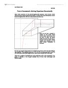
So the first thing to do is to start with an estimate, let us say this estimate is x1. We then draw a tangent of the curve. I.e. we draw the tangent of the curve at the point (x1,f(x1)).
As the equation of a straight line can be written
y-y1 = m(x-x1);
the equation of the tangent must be
y-f(x1) = f’(x1)(x-x1).
Where the tangent cuts the x axis, we will call the point (x2,0), so:
0-f(x1) = f’(x1)(x2-x1).
We can rearrange this to give:
x2 = x1-(f(x1)/f’(x1))
Which gives us the Newton-Raphson iteration formula, which is:
xn+1 = xn-(f(xn)/f’(xn))
When we use our cubic equation with this formula, we can values which will start to converge at a very quick rate, this makes using this formula a lot quicker than using the decimal search with the change of sign method which was explained earlier.
The method with which this is done is illustrated graphically on the next page. Also, on the next page, is the way in which it is possible to find all three roots to the equation.
If we plot this method of obtaining the roots in a table, we get the following:
Where f(x) is applying the function to the value just found. Where f(x) = 0 is where the difference between the tangent crossing the x-axis and the graph crossing the x-axis are the same. The closest we managed to get in this case was 0.00000000000001, which is probably close enough.
So the root is -2.26102917373168 ± 0.000000000000005.
The other two roots are found in these following tables:
The root found in this table is 0.143789558815385 ± 0.000000000000005.
The root found in this table is 2.05057294824819 ± 0.000000000000005.
The error bounds will be 2.05057294824819 and 2.05057294824818
So the three roots of the equation y=3x³+0.2x²-14x+2 are:
2.05057294824819
0.14378955881683
-2.26102917373168
Problems with the Newton-Raphson method
Of course this method is not error free, in fact often when you are searching for a certain root it can be hard to find it as the value you choose as your first x value will return to a root which is not as close to the x value as the root you are actually looking for. This can be a problem in the equation we used above. If you put in the wrong value when searching for a root, you will get one you have already found, and this is best demonstrated when you are looking for the middle root, the one closest to zero.
If you enter a first value of -1, you get the iteration shown below.
Basically, if you enter the value -1, the graph at this point has a negative gradient, and such a value that the line comes down past the next root on the x-axis, and at the place that it meets the x-axis, the graph once again has a positive gradient and so when the second tangent of the graph meets the x-axis, it is actually further away from the expected root than we had imagined, and it has ended up closer to the highest root, which is much closer to two than to zero.
Rearranging the Equation f(x) = 0 into the form x = g(x)
The first step is to change your equation from the form f(x) = 0 into the form x = g(x) as the title itself suggests. For this example we will use the equation:
y=x³-5x+3
so: 0=x³-5x+3
So, the first thing to do is to make x the subject:
5x=x³+3
x=(x³+3)/5
So we have our equation in the x = g(x) form. And this can provide us with the basis for the iterative formula:
xn+1 = (x ³+3)/5
Having rewritten the equation in this form, it means that instead of looking for where the graph crosses the x-axis, we are now looking for where the re-arranged graph crosses the line y = x.
The next step is to do a similar process to what we did in the Newton-Raphson method. We take a first value of x, which we call x1, then we apply the function g(x) to this, and find the point (x1,(g(x1)). We then take g(x1) to be x2, and find g(x2), and we continue until we get to the degree of accuracy which we want. The result on the graph can be seen below, using the original equation in red, y= x³-5x+3; y=x in blue; and the x=g(x) form, in purple:
The solving of the x = g(x) iteration can be seen zoomed in on the next graph.
You can see how the green line, which is the iteration’s graph, moves horizontally, then vertically, as it first finds y=g(x), then moves across to y=x. It results in a step formation getting closer and closer towards the root which is where x=g(x) and y=x meet. We can see that the gradient of the g(x) line has to be between 1 and -1, otherwise the iteration line will start to move in the wrong direction, in this case it is ok, but using other re-arrangements, it might not be.
The table which shows the converging of the two values can be seen below:
We can see that, towards the bottom, the values are getting very close, so we can say that the root’s error bounds are 0.656620431026809 and 0.656620431041859. So we have got very close to the root.
Failure of the x = g(x) Method
It can be very difficult to find one or more of the roots if you use the wrong rearrangement of the equation because of the gradient the rearrangent’s graph will be at when the line crosses the graph of y=x. If the gradient is more or less than 1, the method will find either one of the other roots, or in some cases, no root at all.
If we use the same equation, 0=x³-5x+3, but rearrange it into x=(5x-3)1/3 and then plot it on the same axis as y=x, the gradient of the former equation is greater than 1 when the lines cross. This means that it is impossible to get the middle root as wherever you choose your x1 value, the iteration will plot in the other direction and get one of the other 2 roots.
This problem is illustrated graphically in the graph below.
Comparison of Methods
The other two methods can also find the root found above by the x = g(x) method.
Using the original equation y=x³-5x+3:
Newton-Raphson Method:
Clearly, with this method, the root is found in very short time to be 0.6566204310471 (to 13 decimal places).
Change of Sign Method:
This method also finds the root, but less accurately, and takes more working to get an accurate answer.
It gets 0.6566204 ± 0.00000005 as the root.
Overall Comparison
Overall, all the methods have advantages and disadvantages.
The Newton-Raphson method is certainly the quickest to get to the root, it converges to a point very quickly, and that root can be obtained to many decimal places very fast.
However, to do this at any real speed, you need to have access to a powerful computer program, or be able to do large sums quite fast. It is easy to do if you have a computer program like Excel or Autograph, but otherwise one of the other methods might be easier.
The Change of Sign method is not particularly fast. It does get to a root, but you need to produce whole tables of data for each decimal place you obtain, and this is really quite a slow process. On the plus side, it is possible to do this without any special hardware or software, a calculator and a piece of paper are enough to get to a few decimal places with this method, and if you have the time and patience, you can find many more decimal places.
The x = g(x) method is also slower than Newton Raphson in most cases. It can be quite fast, but it often depends on where you start from, however, assuming you choose a reasonable value, you get quite a good rate of convergance. This method is possible without a computer, but would be very time consuming, and it might be quicker to use the Change of Sign Method.