After 20th terms and approximation of the root to is found. it had an error bound of, in other words it had a solution bound of with a maximum error.
This method can also be shown graphically by computer:
This method can be drawn in software ‘autograph’. By using this program the equation can be enter and there is a function key call ‘bisection iteration’ then we can enter upper and lower bound and this program will be able to help us to find the root automatically.
However this method is not always working properly. There are two situations which lead to the failure of the method
- Discontinuous functions
In this equation, it is discontinuous between Cartesian coordinate (1, 2.8) and (2, 1.63). If my starting value of a and b is 1 and 2 respectively then
However the function of the lower bound is 2.8 and the function of the upper bound is 1.74() and they have no sign change due to it has an asymptote between 1 and 2 therefore there is no sign change and this method will fail when it is not continuous function.
- Close roots
In some cubic function there are 2 close roots and this method will also fail in this situation.
Our target root is between 0 and 1 and if we use 0 and 1 as the upper and lower bound then we will find another root instead of our target root. In this case this method will fail to find the target root we want. If we want to find the target root then we have to set up upper and lower bound very close to the target root in order to find the target root.
- Newton Raphson method
This is a typical method of fix point iteration. The concept of fix point iteration is very similar to interval estimation but instead of bisect two points to find an approximation of roots we will use a ‘fix point’ and try to find a better result from this fix point and eventually it will converge to the roots.
This method requires us to start with a point which is close to the target root and we call it. Then we will find the gradient - at Cartesian co-ordinate and we can find the better estimation - by formula, we can then carry on with the general formula, the sequence will converge and untilit converges to the target root we find.
Example 1
This method can also calculate with the help of Microsoft excel, formulas are set up as following:
n – number of step
- estimation of x
- output of function when x =
- differential of f(x)
- output of when x =
- divide by
- value of next estimation
Target root 1
After 6 converge we can see that the 1st target root is to , with an error bound and solution bound.
Other 2 root are also found:
Target root 2:
After 5 converge we can see that the 2nd target root is to , with an error bound and solution bound.
Target root 3
After 7 converge we can see that the 3rd target root isto , with an error bound and solution bound.
After three solutions were found then we can now create a statement:
‘The equation had 1 solution which comprising 3 roots,
, to. Their error bounds are and their solution bound are, and respectively.’
Newton Raphson’s method can also be shown graphically by computers:
This is part of the equation, I will focus on region because the root is between this region. ‘Autograph’ is also helpful to find a root by Newton Raphson’s method. Gradient can be drawn by autograph easily. We have to use the function – ‘Newton Raphson iteration’ and choose the value of then a gradient will be drawn by this software automatically. This is efficient way to find the target root without too much process.
However there are situations which this method fails:
Discontinuous function
A spread sheet had also been set up for help:
After 5 steps the sequence becomes and it is clearly that this sequence is diverging to. This is an example of failure case to Newton Raphson’s method.
The reason is because the gradient –f'(xn), the gradient is so small and on the process f(xn)/f'(xn) it becomes infinitely large and consequence xn+1 is very large and this value diverges to infinity.
-
Rearrangeinto form
This is also a method by using fix point iteration and algebra was also involved. The basic concept is arrange into a new form - and we can then derive two equations – and. We can then able to solve by determine the intersections of two equations and also with the help of fix point iteration.
:
This equation had infinity number of arrangement, therefore one of them will be chosen by myself and I choose two new equations and they are and respectively. They are then shown by computer graphically:
Then we set up a fixed point - and it can be any value but near to the target root and we are able to find a better approximation call, this sequence can repeat and eventually estimations approach to the target root will be found.
Microsoft Excel can also helpful and therefore a spread sheet is set up:
-number of iteration done.
- value of x
- output of x when
- gradient of xn
After 18th iteration the root approach to to and there is error bound and solution bound. Gradient is also calculated because it had to obey restriction. In this case it is -0.625 which means the root can be found and the sequence converges.
Can other arrangement work?
There are many ways to rearrange, and are only one way to rearrange this equation, but can other rearrangement find the same target root? Another rearrangement is done:
A graph is then drawn in computer
If we out starting value as 0 then is converge to another root but not target root, therefore we use starting value 1 and it also converges to another unexpected root therefore this rearrangement fails to find target root.
Excel spread sheet had also set up for observation:
This proves furthermore both starting value do not converges to the target root and in this case it cannot be use to find the target root therefore it is fail in this situation and we have to decide which rearrangement is work in order to find the target root.
How about other roots? Can this method use in order to find other roots in?
If 2 is apply tothen the target root is not found, instead another root is found then I apply 3 to then something strange happen as shown:
This sequence is not converging to the target root but instead it diverges to infinity. To prove this furthermore a spread sheet is set up to give more evidence
After 4 iteration the sequence is clearly to diverge to infinity because numbers is getting very large. On the 4th sequence g (xn) is so large that even computer grid cannot show the value ( it appears as ############ which means there is no space to show the value of g(xn).). We can then consider to the gradient and one conditions shows why method is fail.
The reason why it is not work is because there is one restriction – the gradient of, cannot be greater than 1 or less. In other words if the gradient is greater than 1 then iteration is not found due to the sequence diverges instead of converges.
This can be shown by
When, and .its modulus value (0.625) is smaller than 1 therefore this iteration is working properly and converges to root.
However if, and, this is much greater than 1 therefore this iteration is not working properly and diverges to infinity.
Compare and contrast between these three methods
At the starting point, I will choose one equation I have use before and the choice from me is equation , one root of this equation have been find by method of rearrangement to form and it is. To compare and contrast three methods I have to find this root again by using other method and see which method gives a better result, less time consuming and ease of use with available hardware and software.
Method of Bisection:
Newton Raphson’s method
,
Rearrange into form
,
Let us focus on the speed of converges at the first place. It’s clearly that Newton Raphson’s method is the quickest way to find a root in this example. It takes converges and unlike other two methods they take at least 15 steps to converges to the root..
Error is very small in all 3 situations because it is correct to and the error bound is therefore the error is relatively small. There is a slight disagreement of the root between rearranging method and other two methods. The rearranging method states that the root is and the other two methods states it is. But there is onlyerror between two roots therefore the error is relatively low in this case.
Table compares and contrasts between three methods