Error Bounds
We can therefore establish that the smallest root of the equation is -1.4119815 with a maximum error bound of ±0.0000005.
Failure of the method
If I take as the starting value x0 = 0 to find the value of the other 2 roots of this equation, then a problem is encountered. This is because when I do the calculations, increasing x by step of 1 unit, the roots will be missed as no sign change in the value of f(x) occurs from x = 0 to x =1 ( as shown below).
Newton-Raphson
This method involves fixed-point estimation, whereby a tangent to the curve from an initial value of x is drawn then it is calculated where the tangent intercepts the x-axis… this gives a better approximation to the root. Repeating the process gives more and more accurate values for the root until the desired accuracy is reached.
The equation that I have chosen to solve is x5 – 2.1x + 0.6 = 0
Newton-Raphson formula is:
The iterative formula is:
The graph below illustrates y = x5 – 2.1x + 0.6.
The graph on the following page illustrates y = x5 – 2.1x + 0.6 and it shows the effect of drawing successive tangents from a starting value of x0 = -1.5.
This illustration demonstrates how we acquire the first root of the equation. The tangent is found at a point and then the point where this tangent crosses the x-axis is found. In the table below, x is the approximation to the root and |Δ| is the modulus of the error.
x |Δ|
-1.33441057 0.16559
-1.274151543 0.060259
-1.266706903 0.0074445
-1.266601067 0.000105795
-1.266601067 2.11252E-08
From the various calculations, x0, x1, x2, … converge on the root –1.266601067 in 5 iterations. The other 2 roots were found in the same way, repeating the same operations.
The graph below illustrates y = x5 – 2.1x + 0.6 and it shows the effect of drawing successive tangents from a starting value of x0 = 0, in the scope of showing how to find the root near x = 0.5.
From the various calculations, x0, x1, x2, x3 … converge on the root 0.2866356508 in 4 iterations.
The graph below illustrates y = x5 – 2.1x + 0.6 and it shows the effect of drawing successive tangents from a starting value of x0 = 1.5, in the scope of showing how to find the root near x = 1.5.
From the various calculations, x0, x1, x2, … converge on the root 1.118199046 in 6 iterations.
Therefore the 3 roots are:
- –1.266601067 found in 5 iterations
- 0.2866356508 found in 3 iterations
- 1.118199046 found in 6 iterations
Error Bounds
To check the error bounds I have found y for the x values equal to -1.26660106, and -1.26660107. The results are shown below:
- when x = -1.26660106, y = negative
- when x = -1.26660107, y = positive
This shows that there is a change of sign and therefore:
x = -1.266601065 ± 0.000000005
Failure of the method
The method fails if the initial value is not close to the root, or is near a turning point of y = f(x), the iteration may diverge, or converge to another root.
The equation that I have chosen to solve is x5 + 2.1x4 + 0.8x3 + 0.7x2 – 0.4x – 0.9 = 0
To demonstrate the failure of the method I have decide to take a starting value of
x0 = 0 and therefore to find the root between x = -1 and x = 0. For the equation
y = x5 + 2.1x4 + 0.8x3 + 0.7x2 – 0.4x – 0.9, dy/dx = 5x4 + 8.4x3 + 2.4x2 – 1.4x – 0.4, therefore if x0 = 0, dy/dx = -0.4.
As we can notice, the gradient of the tangent is negative. And as shown below in the graph, the Newton – Raphson method converges to the root close to x = -2 (which is the furthest from the starting value x0 = 0).
Fixed Point Iteration
In this method the equation f(x) = 0 is re-arranged in the form x = g(x). A root of the equation is seen as where the line y = x and y = g(x) intersect. Using the formula f(x)=0 another formula g(x) = x is derived, and the root can be found of the equation.
The equation that I have chosen to solve is x5 + 0.5x2 – x + 0.1 = 0
Re-arranging the formula to get the equation in the form of x = g(x). One of the many different forms of the equation is x = x5 + 0.5x2 + 0.1
The graph below illustrates y = x5 + 0.5x2 + 0.1
The graph below shows y = x and y = x5 + 0.5x2 + 0.1 and shows the convergence with a ‘staircase’, where x0 = 0.5 as the starting value for iteration.
This graph on the previous page demonstrates more clearly how we acquire the root of the equation.
From the various calculations, x0, x1, x2, … converge on the root 0.105588 in 8 iterations.
Differentiation of g(x):
g’(x) = 5x4 + x
If the root is x = 0.105588, then g’(x) = 0.1062…
g’(x) < 1, therefore this root is not as steep as the gradient of y = x, and therefore it will converge.
Failure of the method
To demonstrate the failure of the method I will try to find the root near x = 1, using the same rearrangement but taking a different value as starting point, which is x0 = 1.
The graph below shows both y = x and y = x5 + 0.5x2 + 0.1 and shows how the fixed point iteration method fails with x0 = 1 as the starting value.
The graph clearly shows that the staircase diverges away from the intersection of the two graphs, i.e. is not converging, and therefore the root near x = 1 won’t be found. This demonstrates the failure of the method.
From the spreadsheet it can be seen that there is no converging towards a root, in fact the x value increases so much that it is too big for the computer to calculate.
Because the method is applied to the same rearrangement of before, g(x), this clearly show a failure of g(x) fixed point iteration.
Differentiation of g(x):
g’(x) = 5x4 + x
If the root is x =1, then g’ = 6.
g’(x) > 1, therefore this root is more steep than the gradient of y = x, and therefore it will diverge.
Comparison of the three methods
To compare the three methods I will attempt to find the middle root of the equation:
x5 + 0.5x2 – x + 0.1 = 0
This equation is also the equation that I have solved with the fixed point iteration method. I will find the middle root because otherwise there will be a failure in the fixed point iteration method, as shown above.
The graph below shows the equation y = x5 + 0.5x2 – x + 0.1
Using Fixed Point Iteration Method:
The root of this equation was 0.105588, and was found in 8 iterations.
Using Decimal Search Method:
I am taking x0 = 0 as my starting value but instead of adding 1 to x0 I will add 0.1 otherwise no root will be found.
The calculations have been done using Excel and are shown below.
The root obtained is between 0.105588 and 0.105589. Therefore the middle root of the equation is 0.1055885 with a maximum error bound of ±0.0000005. To achieve this answer it took 35 iterations.
Using Newton-Raphson Method:
I am taking x0 = 0 as my starting value.
The graph below shows how we acquire the middle root of the equation.
From the various calculations, x0, x1, x2, … converge on the root 0.105587 in 4 iterations.
To summarize, the three results were as follow:
- Decimal Search Method = 0.1055885 in 35 iterations
- Newton-Raphson Method = 0.105587 in 4 iterations
- Fixed Point Iteration Method = 0.105588 in 8 iterations
From the 3 results shown above, I can clearly conclude that the Newton-Raphson method is the quickest one, because it gives the fastest convergence. It does reply on being able to differentiate the f(x) though.
The Decimal Search method is very tedious because it takes a lot of time to prepare the spreadsheet on Excel: especially the various formulas for the different calculations. And as shown above it takes many iterations to find the root.
The Fixed Point Iteration method takes a lot of time to find the right rearrangement of an equation, because not all g(x) graphs will allow convergence to the required root. I had also problems using the software Autograph, because when I had to load the method, it didn’t work for the first few times. As shown above it takes 8 iterations. This time the number of iterations required was very small as it usually takes many more (and depends on the value of the gradient of g(x) near the root) – the closer this is to 1, the faster is the convergence.
The Newton-Raphson method requires much less time for the preparation than all the other methods, and is definitely much simpler. With just a click on the graph it shows exactly the number of iterations and it shows on the graph the various tangents. It’s the fastest method, especially because it required only 4 iterations to find the middle root of the equations.
To conclude, the Newton-Raphson method is the best between the three, because it’s quick and very easy to use.
P2 Coursework by Francesco Egro