Results:
In this graph, the gradients at these points alter. The -1 on the x axis has a gradient of 3. The gradient of the straight line is positive.
-Now, I will investigate the set of graphs which include parabolas.
The set of graphs which I will investigate will have an algebraic equation:
y=axn
The graphs which I will investigate are:
I will investigate all of these graphs firstly using the Triangle Method and then comprise other methods such as the Increment Method.
I will begin by drawing the table of values, and then finding the results of the graphs.
‘y=x2’ solved by the ‘Triangle Method’
This graph will have a parabola, as it is a graph of a quadratic equation. The powers in quadratic equations are always greater than 1. This graph will be at a minimum curve. When a curve is at a minimum it always encompasses a gradient which goes from a negative to a positive.
y=x2 is a minimum curved graph.
Results
From this graph, the results achieved are not absolute accurate, this is due to the graph plot. But as you can see the results do make some sense.
In this graph I begin to see a pattern in the gradients. I have investigated the following points in the ‘x’ scale; 3, 4 and -2.
From looking at the graph results, its seems like the ‘x’ values are being doubled (multiplying by 2). If we round the gradients down to their lowest term, the gradient would look as follows:
As you can see above, the ‘x’ value has been doubled, that gives you the gradient for the points in the graph ‘y=x2’.
I will now incorporate more graphs into my investigation. I will also start to solve different graphs by the Tan θ method. This method is very similar to the Triangle method. Here is an example how to use the Tan θ method:
Tan θ method
The Tan θ method is very similar to the Triangle method. It is not as accurate as the Increment method, but can be used to give an estimate of the gradients.
First of all, you will need to draw a tangent on the curve. Then similar like the Triangle method, you need to draw the ‘x’ and ‘y’ differences. The purpose of this method is to find the angle in the right angled triangle. It is a trigonometry method you will need to use.
The method is: Angle = _ Opposite
Adjacent
This is the Tan function in Trigonometry. This is why it is called the Tan θ method.
So the angle equals = 16
2.2
= 7.27˚ [this is also the approximate gradient for x=4].
‘y=2x2’ solved by the ‘Tan θ Method’
I will now go on solving more complex quadratic graphs such a ‘y=2x2’.
Results
Values at point:
2: x= 1.15, y=9 [9/1.15]
3: x= 1.45, y= 18 [18/1.45]
4: x= 1.9, y= 32 [32/1.9]
-2.5: x= 1.3, y = -12 [-12/1.3]
-4: x= 1.8, y=-32 [-32/1.8]
Above are the differences in the ‘x’ and ‘y’ scales.
As you can see, I have investigated all the positive points on the ‘x’ scale. Some results are not all to 1 decimal place. The pattern in this results table is that the ‘x’ value has been multiplied by 4. If you round the values up and down to their lowest terms and highest terms, they will equal to the following:
x=2: 7.82 (round up to 8) the 2 has been multiplied by 4.
x=3: 12.41 (round down to 12) the 3 has been multiplied by 4.
x=4: 16.8 (round down to 16) the 4 has also been multiplied by 4.
x=-2.5: -9.23 (round to -10) the -2.5 has been multiplied by 4.
x=-4: -17.77 (round down to -16) the -4 has been multiplied by +4.
These results are not exactly accurate due to the graph scales, but they show an approximate of how close they are. The gradients obtained are all multiples of 4.
The Increment Method
The increment method is another method which calculates the gradient of a line. This method is much more accurate than the ‘triangle method’.
Here is an example of how to use the Increment Method:
The first thing you need to do is to draw the tangent across the point you want to calculate. (In my case, x=4). After you have done that, then draw down the line of differences.
After you have done that, on the ‘x’ axis you have to move across to a value which is very close to your previous ‘x’ value. (In my case, x=4; move to 4.01). After you have done that, then square that number and then the value you get from that draw a line from that point on the ‘y’ axis. [4.012 =16.0801]
Once you have done that you will need to make a very small triangle between the two lines and then zoom up on the triangle either using a glass rod or something relevant. Once you have zoomed up you will see that the curve has become so small that it seems as a straight line. You will then need to find the differences between the lines. You can do this by the following method:
Differences: change in y = y2-y1 [16.0801-16]
change in x = x2-x1 [4.01-4]
After you have found the differences, you will need to do:
y difference
= [0.0801]
x difference [0.01]
So the gradient equals to 8.01= 8.
The Increment method is a very accurate way of finding the gradients.
‘y=x2’ solved by the ‘Increment Method’
I am now repeating this graph by using the Increment Method.
Results
For each of the ‘x’ points, the increment which I moved to was ‘0.01’. Each point at which I found the gradient was to an increment of 0.01. I have showed the results with a zoomed up triangle. The results were more accurate than the ‘triangle method’.
Gradient for the points:
x=1
x1: 1 y1: 1
x2 [Increment]: 1.01 y2: 1.0201 [x2 squared]
y2 – y1
= Gradient
x2 – x1
Gradient = 1.0201 – 1
1.01 – 1
= 2.01
The gradient of 1 is 2.0 to 1.d.p.
x=-2
x1: -2 y1: 4
x2: -2.01 y2: 4.0401
Gradient = 4.0401 – 4 = 0.0401
-2.01 - - (+) 2 = -0.01
= -4.01
x=-4
x1: -4 y1: 16
x2: -4.01 y2: 16.0801
Gradient = 16.0801 – 16 = 0.0801
-4.01 - -4 = -0.01
= -8.01
x=3
x1: 3 y1: 9
x2: 3.01 y2: 9.0601
Gradient = 9.0601 – 9 = 0.0601
3.01 – 3 = 0.01
= 6.01
The results obtained above are very accurate. The gradient of the graph ‘y=x2’ is just 2 multiplied by the ‘x’ value. If the value is negative then the gradient will also be negative, because the negative value is going to be multiplied by +2, so the result will be negative.
Now, I will solve the following graphs using the Increment method:
‘y=x3’ solved by the ‘Increment Method’
I am using the Increment Method, because this graph has a very awkward curve which is hard to find the gradient, so I will need to be a specific as possible and use a method which will calculate the gradient accurately.
The graph follows on the next page
Results
x=1:
Gradient = 1.030 – 1 = 0.03
1.01 – 1 = 0.01
= 3
x=2:
Gradient = 8.120 – 8 = 0.12
2.01 – 2 = 0.01
= 12
x=3:
Gradient = 27.27 – 27 = 0.27
3.01 - 3 = 0.01
= 27
x=4:
Gradient = 64.48 – 64 = 0.48
4.01 – 4 = 0.01
= 48
These results obtained are very accurate. They have no decimal places.
‘y=2x3’ solved by the ‘Increment Method’
This is another cubic graph, but it is more complex than ‘y=x3’
Graph on next page
Results
x=1:
Gradient = 2.060602 – 2 = 0.060602
1.01 – 1 = 0.01
= 6.0602
x=2:
Gradient = 16.24 – 16 = 0.24
2.01 – 2 = 0.01
= 24
x=3:
Gradient = 54.54 – 54 = 0.54
3.01 – 3 = 0.01
= 54
x=4:
Gradient = 128.96 – 128 = 0.96
4.01 – 4 = 0.01
= 96
‘y=x4’ solved by the ‘Increment’ method
Results
x=1:
Gradient = 0.0406 / 0.01 = 4.06
x=2:
Gradient = 0.3224 / 0.01 = 32.24
x=3:
Gradient = 1.085 / 0.01 = 108.5
x=-2:
Gradient = -0.3224 / 0.01 = -32.24
I will now go onto more complex graphs such as:
‘y=x 1/2’ solved by the Increment Method’
This graph ‘y=x1/2’ gives values of the square roots of the ‘x’ values. This graph will have no negative values because there is no square root of a negative number, therefore the graph will only cross through the positive axis.
Results
x=1:
Gradient = 1.0049 – 1 = 0.0049
1.01 – 1 = 0.01
= 0.49
x=2:
Gradient = 1.417 – 1.414 = 0.003
2.01 – 2 = 0.01
= 0.3
x=3:
Gradient = 1.7349 – 1.7320 = 0.0029
3.01 - 3 = 0.01
= 0.29
x=4
Gradient = 2.0024 – 2 _ = 0.0024
4.01 – 4 = 0.01
= 0.24
The results of y=x1/2 are very different to any other graph. The gradient in this graph decreases as the ‘x’ values increase.
‘y=x-3’ solved by the ‘Increment Method’
Results
x=1:
Gradient = 0.9705 – 1 = -0.029
- – 1 = 0.01
= -2.9
x=2:
Gradient = 0.1231 – 0.125 = -0.0019
2.01 – 2 = 0.01
= -0.19
x=3:
Gradient = 0.036669122 – 0.03703704 = -0.000367
3.01 – 3 = 0.01
= -0.0369
The gradients here vary. They become smaller and smaller as the ‘x’ value increases. The x=3 has a very small gradient. This graph is very complex and is difficult to solve with the ‘Tangent Method’ so therefore I have used the Increment Method.
Now I am heading towards the final part of my investigation. I am now going to introduce a concept of a ‘limit’. I have looked this up in an A-Level mathematics textbook called:’Pure Mathematics 1’.
Limit
The basic concept of a limit is very similar to the Increment Method. It involves the same method to obtain results. A limit is a very small increment in an ‘x’ value. It involves the usage of a Greek letter ‘δ’. This is pronounced: D-e-l-t-a.
Below is an example of how to use a limit:
Like the Increment method, you need to draw down the differences, and then move along a very small increment. The increment which you move along will be replaced by the Greek letter: δx, so now that increment will become for example: 3+δx, instead of 3+0.01= 3.01.
You will then need to find the differences of the triangle as you do in the Increment method.
Gradient = 6δx+ δx2
δx
= 6+ δx
So the final answer you will get the gradient of the point and the small increment which you moved across the ‘x’ value. To find the difference in δy, you needed to ‘square’ the ‘x’ value + δx.
So the definition of a limit is that it is the ‘small increment’ which you move across the ‘x’ value during the Increment method. This limit can be used as any symbol, but is commonly used as ‘δ’ or ‘Δ’.
The gradient of a curve is usually written in a notation of
δy
δx
Maximum and Minimum curves
There are usually 2 types of gradient curves. These gradient curves are called, maximum and minimum.
These curves represent the gradient of a curve when it reaches the maximum and minimum points, and the gradient becomes zero.
Below are examples of some Maximum and Minimum curves:
Above is an example of a minimum curve. The curve crosses through the positive points of the y axis. The gradient is at zero at the bottom. Minimum curves have a gradient of zero at the bottom of the y axis.
This curve is at a maximum. The curve crosses through the negative points of ‘y’. The gradient of zero is at the top of the y axis.
These are the two types of curves. A minimum curve is created when the equation is all positive for example: y=x2. This shows you that the curve will be crossing through the positive points of ‘y’.
A maximum curve is created when the equation has a negative value of ‘x’. For example: y=-x2. The curve will cross through the positive points of ‘y’.
Suggesting a formula
I will now suggest a formula for the gradient of a curve, but firstly I will look at number sequences of the graph equations. I will then talk about ‘Differentiation’. This is another topic which I looked up in a Mathematic A– Level textbook.
2 4 6 8 10
2 2 2 2 Formula: 2n
y=2x2
4 8 12 16
4 4 4 Formula: 4n
y=x3
3 12 27 48
- 15 21
6 6 Formula: 3(n2)
y=2x3
9 36 81 144
27 45 63
-
18 Formula: 9(n2)
y=x2
For this equation the gradient is 2x. Turning x2 into 2x I will need to find a method.
y=x2:
This equation has a power of 2, but 2x has a power of 1. So therefore the power of 2 has been taken by 1 and it seems if the power has been put in front of the x value, so its been subtracted by the 1 and then put in front of the x value.
So now that gives me a hint of what would happen to the equations. They will need to be re-arranged and the powers will need to be taken away by 1.
Let me test other equations for this same method.
y=2x2
To find the gradient for this equation the ‘x’ values are being multiplied by 4.
So if I use my method to work this out it will look like this:
x=1 = 2 x (multiplied) by 2 x (multiplied) by the x value (1) = 4.
x=2 = 2 x (multiplied) by 2 x (multiplied) by the x value (2) = 8
So it seems like my method is working for both equations.
I will now test it for y=x3
y=x3
y=3x2 (this would be the new formula). The power has been subtracted by 1 and the previous power has been placed in front of the ‘x’.
So now that I have tested and worked with my method, I will need to simplify it a little.
Step 1:
For example: y=x3
Subtract the power by 1. So then that becomes:
y=x3-1
Step 2:
You will need to bring the previous power in front of the equation. So that becomes y=3x3-1
So the final equation becomes:
y=3x2
And if we want to test this method for a different equation, for example:
y=4x2
If we want to find the gradient for the x value of 2, the method would work like this:
Y=4x2
= y=2 x 4x(x=in our case 2)
So that is y=2 x 4 x 2
= 16
The gradient for the ‘x’ value 2 is = 16.
This is where ‘Differentiation’ has taken place. I have differentiated the equations into a simple formula = nx n-1
‘n’ being the power and ‘x’ the value of the equation. Differentiation is the co-efficient placement of the power in the equation.
In the beginning of my investigation I was achieving the gradient function by the tangent method. However, when progressing throughout the investigation, it became very clear that the tangent was not necessary in finding the gradient function of a graph, as the increment was enough to prove that alone.
Progressing further along using the concept of a ‘limit’ showed that there was a formula which gave the gradient of a curve.
At the last stages, I have used number differences to obtain different formulae for different equations. Each stage of investigating got closer and closer to the algebraic formula, which is:
nx n-1