The normal distribution
When many measures are taken of something (eg, scores in a test, people's heights, pollution levels in rivers) the spread of the values will have a bell shape, called the normal distribution.
A number of statistical tests use this characteristic distribution (or dispersion) of values to test whether two samples are the same or different.
There are several basic terms that are commonly used with the normal distribution.

Standard deviation
The normal distribution at right shows the percentage of scores/observations that lie within one, two or three standard deviations either side of the mean. That is, 68%, 95% and 99.7%.
The 95% value, which is used as the standard in tests of significance) lies between 1.96 standard deviations either side of the mean.
Standard deviation of a sample
is the squared difference between each score and the mean
Σ means the sum of all the squared differences (add them all up)
n – 1 ...
This is a preview of the whole essay
Standard deviation
The normal distribution at right shows the percentage of scores/observations that lie within one, two or three standard deviations either side of the mean. That is, 68%, 95% and 99.7%.
The 95% value, which is used as the standard in tests of significance) lies between 1.96 standard deviations either side of the mean.
Standard deviation of a sample
is the squared difference between each score and the mean
Σ means the sum of all the squared differences (add them all up)
n – 1 means the number of scores minus 1
The table below shows how to calculate the average and the standard deviation of a set of seven example scores in the first column. The average is 39.93 and the standard deviation is 2.73.
Comparing two samples: using the t test
The average, standard deviation and the number of scores in each sample are the three things needed to do a t test. A t test is used with two samples of data to test whether they are significantly different (ie, whether one is truly higher or lower than the other). The same sample of scores as used above is now compared with another sample of scores.
- Put the values into the equation and work it out carefully!
- Note down the value of t found. In this case it is 3.08.
- You will also need to know how many degrees of freedom to use with the critical values of t table. Degrees of freedom = (nsample1 + nsample2) – 2 . In this example this equals 7 + 7 –2 = 12.
- Find the value of t for that number of degrees of freedom using the table supplied (it is 2.179). Since the value calculated for your data is higher than it the difference is judged to be significant/real (at the 5% level). That is, the difference between the samples has less than a 5% chance of occurring by chance (being a fluke).
It doesn't matter if the value of t is negative or positive: just use the positive value to work significance.
Mathematics assignment (Due 12.00 pm Monday the 13th January 2003, and must be handed in to Jeanette Bray or Jean Worrell at the Help Desk in UH 255). I need to see how each question was worked out. I will not give marks for answers without calculations. I will be available for revision for the exam in GN101 10-12 and 2-4 on Fri 3rd.
1. The relationship between wombat weight and their production of methane gas is shown below.
- Draw a line of best fit through the data points and use it to derive the equation for the line (y = mx + c).
- Rearrange it to solve for x. That is x = …………………..
- Use the equation from part b to predict the weight of a wombat that produced 12.2 mg methane per hour.
2. Calculate the average, range, median and mode for the following set of data (a random set of your exam results from the last exam): 66.25, 15, 32.5, 26.25, 48.75, 48.75, 36.25, 35, 68.75, 72.5, 43.75, 40, 20, 48.75, 12.5, 41.25, 53.75, 50, 31.25, 95, 22.5, 33.75, 27.5, 55, 12.5, 45, 18.75, 42.5, 62.5, 85, 75
3. The two sets of data given below are resting heart rates for a group of students and a group of professional athletes. Use the t test to find out if they are significantly different (using the table at right to test the value of t with the appropriate number of degrees of freedom). I need to see how the mean, standard deviation and t value were calculated.
Professional
Students athletes
57.1 61.7
47.6 47.0
58.0 55.5
74.8 62.6
- 41.8
51.9 60.8
64.2 50.2
49.6 44.2
67.2 45.4
62.6 39.3