n And, this will be used along with the mean of the sample to create confidence intervals for the mean of the parent population of smarties.
n Also, calculations that determine the size that a possible sample could be to achieve a certain percentage confidence interval for the mean to be a certain range.
Accuracy of measurements
The smarties will be weighed on an electronic balance that will be “reset” to zero after each measurement to reduce any chance of any inaccuracies that might arise from small pieces of smartie being left on the balance.
The balance available gives measurements in grams, to three decimal places. This seems to be an acceptable level of accuracy, as it is not too high to be inefficient, and not to low as to be too inexact and affect the data. However, if the difference in the weight of smarties is too small to be detected on this balance, either a more accurate balance must be found or a survey of something with a higher variance must be carried out.
Results (sample data)
Mean, Standard Deviation and Variance of Sample
Estimate of the Variance of the Population of Smarties
The variance of the sample is a biased estimator. A biased estimator is one for which the mean of its distribution is not equal to the population value it is estimating. To convert the variance of the sample to an unbiased estimator it must be multiplied by where n is the size of the sample.
This figure can then be used to estimate the variance of the parent population.
Standard Error
The standard error is the standard deviation of the sample mean. According to the central limit theorem, the variance of the sample mean can be calculated by dividing the variance of the population (estimated above) by the size of the sample. The standard error can be calculated by performing a square root of the variance of the mean. This can be demonstrated algebraically:
Estimate of the Mean of the Parent Population
The mean is an unbiased estimator, that is, the mean of its distribution is equal to the mean of the parent population. For this reason it can be used as an estimator for the mean of the population of smarties. An estimate of the mean of the population of smarties is therefore 0.976.
The standard error calculated above is quite small. This means that the variance of the sample mean is low, and this shows that one can be quite confident that the actual mean of the population is around 0.976. However this is not a very “mathematical” or “user friendly” method of showing how confident one is about the accuracy of the estimate made.
Confidence Intervals Background
To calculate how confident one is about the estimate of the population mean, one can use confidence intervals. These tell you how confident (as a percentage) you can be that the mean of the population falls within a given range. How they work is explained in the following.
According to the Central Limit Theorem, the sample mean is distributed Normally. The mean of the sample mean (the centre of the curve) is equal to the population mean. The shaded area in the diagram shows the population mean ± 1 standard error. According to the tables for the normal function, this comprises of 68% of the curve. This means that there is a 68% chance that the mean of the sample is within one standard error of the mean of the population. This probability can be written algebraically as an inequality:
However, as m is not known when sampling, the above inequality is useless, as it is not known to which number to add or subtract the standard error from. So the
inequality is rearranged thus:
This shows that the probability that the population mean is within 1 standard error of the sample mean is 68%. In other words you can be 68% confident that the population mean is within 1 s.e. of the sample mean.
This idea can be used to calculate the confidence intervals that allow you to be 90%, 95% and 99% sure of the range where the population mean is found.
Confidence Interval Calculations
90%
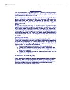
To work out a 90% confidence interval, you must work out how many standard errors from the mean contain 90% of the area under the curve (shown by the 0.9 in the shaded area above, as the are under the whole curve is equal to 1). The table of the Normal function shows areas to the left of points on the x-axis. This means that to work out the z score (the number of standard errors), you must calculate the total area to the left of the “z”, and look that up in the table to find the z score. This then allows you to calculate the confidence interval:
This in words means that you can be 90% confident that the mean weight of the population lies between 0.936g and 0.989g.
The above method is followed for the next two confidence intervals.
95%
This means that you can be 95% confident that the population mean is between 0.961g and 0.991g. This is a larger range than that of the 90% confidence interval, because to be more confident, the possible range must increase.
99%
This means that you can be 99% confident that the population mean is between 0.956g and 0.996g.
Further Confidence Calculations
If I wanted to be 99% that the population mean was ± 0.001g of the mean of the sample, I would have to take a larger sample.
The z score for 99% is 2.575. To obtain the confidence interval (such as the ones calculated above), I would have to multiply this figure and by the s.e. and add it to or subtract it from the sample mean. However, now I have the confidence interval, and I am trying to work out the correct size of the sample so that the standard error is small enough to have a very small confidence interval. In essence I am doing the process backwards.
This calculation just completed depends on the fact that the variance of the population is the variance estimated using the previously collected sample.
The above shows that to create a very small and “confident” confidence interval, a very large sample is needed, of about 20,000. This is not practical, and as far as can be seen at the moment, is a waste of time at least when total accuracy is not needed.
Conclusion
Here are the population parameters that have been estimated:
Variance = 0.00305
Standard Deviation = 0.0552g
Mean = 976g
Confidence Intervals for the Mean:
90% = 0.936g < m <0.986g
95% = 0.961g < m < 0.991g
99% = 0.956g < m < 0.996g
Limitations
The size of the sample was small. The calculations that relied upon the data collected are therefore inaccurate to some extent. To be more accurate a large sample must be collected. Accuracy in the realm of to 0.001g is unlikely to be needed, so a larger sample would not necessarily have to be as big as 20,000, which is very impractical
The sample might have been a “fluke” I might have got all the big smarties, or all the small ones. However there is not much to do to eliminate the possibility of this apart from to weigh every single smartie. This is extremely impractical (possibly impossible).
The smarties gathered were from my immediate area. Even though they were taken from different shops and different packets, they do not necessarily represent all the smarties in the world, only ones in my area.
The results may be unreliable because the company that produces smarties may be changing, or have changed the mean weight setting for the smarties. They may be trying to slowly lower the weight while keeping the price the same. This could mean that the actual population parameters are somewhat different to the ones estimated here.
Possible Extension
A statistical analysis of entire tubes of smarties could be carried out. The actual weight of the smarties could be compared to the price on the tube to determine whether the manufacturers are lying about how much smartie there is in their packets.
Weighing smarties of different colours could also be done to find if there are any differences between them.
Also, a larger sample size could be taken to determine the mean and variance more accurately