I have included a class list on the next page to demonstrate how the males and females were numbered separately.
Pilot Survey
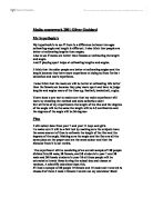
Before carrying out the main investigations I conducted a pilot survey to test if my proposed method would work efficiently. This is done to discover any problems in the method used on a smaller scale-instead of testing a large number of people we instead tested only 5 boys and 5 girls from my maths group.
Pilot Survey Analysis
Our pilot has revealed that there are some problems with the way we had originally planned to collect our data.
Our first mistake was allowing candidates to see other people’s estimates. This caused many people to cheat and so our results were inaccurate. Instead of letting everybody inside the room at the same time we should make the candidates form a line outside the classroom and let them inside one at a time to be tested. There should be one person from our group stood outside the classroom during this time ensuring that no information is passed between candidates as they enter/leave the room.
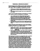
We should also change the way in which candidates are presented with the measurements they will be estimating. Instead of both angles being on one piece of paper they will be drawn on separate pieces of plain paper using a black marker pen and a ruler. The lines of the angles will be of equal length. These steps will be taken to make sure that the measurements are clear and the candidate’s attention is only on one measurement at a time. The instructions given to the candidates should be the clear, constant and also outline the units in which they should estimate and how many decimal places (if any) their estimates should include. This will ensure that all candidates are provided with the same amount of information before they give their estimates and also that no confusion occurs. I think that there should be a time limit as to how long each candidate is allowed to see the measurements for, as it is unfair if one person takes longer than another at thinking of their estimates. There will be a limit of 10 seconds.
I have decided that for my actual results table I will not use percentage error as I feel it is an unreliable method of comparison. This is due to the fact that it does not give proportional results, e.g. an error of 5˚ from 52˚ is 10%, where as the same error for 156˚ becomes 3%. Instead I will just use absolute error.
Hypothesis 1 Results Table Analysis
I think that overall the results I recorded for my first hypothesis support my idea that it is easier to estimate the size of an acute angle than an obtuse angle. The mean estimate of the acute angle (which was actually 52˚) came to about 52˚. The mean estimate of the obtuse angle (which was actually 156˚) came to about 149˚. The mean absolute error for the acute angle came to about 4˚, and the mean absolute error for the obtuse angle came to about 14˚. I think that the mean values for the absolute error of both angles back up my hypothesis the best, as they show a larger range (10˚) than errors shown when mean values of the estimates were worked out (about 3˚). I don’t think that the mean estimates give a very good idea of the accuracy of estimating as it is worked out using a large range of numbers (acute angle: 45˚-64˚, obtuse angle: 27˚-175˚), but the fact that the mean actual estimate for the acute angle is the same as the actual value gives strong evidence that my hypothesis is probably true. However, I believe the mean absolute errors to be more accurate as there is a smaller range of numbers used in the calculation, (acute angle: 0˚-12˚, obtuse angle: 0-129˚).
The mean values I have calculated for the obtuse angle will have been greatly affected by the anomalous result of 27˚, which I have highlighted in my results table. When the anomalous result is left out of the calculations the mean estimate becomes about 153˚, and the mean absolute error becomes about 10˚. This seems to make my hypothesis a little less true as the margin of error becomes smaller. However, I think that the fact that an anomalous result was recorded as an obtuse angle estimate backs up my hypothesis even more. It probably occurred because the candidate found it very difficult estimating the obtuse angle, as their estimate for the acute angle was only 3˚ out.
The modal values for each angle size also back up my hypothesis, as the errors for the obtuse angle are much greater than those of the acute angle. (The difference between the 2 absolute error modal values is 11˚).
Hypothesis 2 Results Table Analysis
I think that overall these results support my hypothesis, however the difference between the two sets of data is not as large as I had originally thought they would be. In this case both sets of mean values back up my hypothesis, but the modal values refute it. The mean value of the line (which actually measured 13.7cm) as estimated by Year 7 was 11.45cm, but 12.87cm for Year 11 students. This shows that the Year 11 estimates were more accurate. The mean values of the absolute error for both year group samples were about 3cm for Year 7 and about 1cm for Year 11. This also proves my hypothesis to be correct, however there is only a range of 2cm. The modal values for each year group prove my hypothesis to be false, as they show that the Year 7 students were the more accurate estimators. However, the values that display this do not have a big difference-the modal values of actual estimates have a difference of 0.5cm, and the modal values of the absolute errors have a difference of only 0.1cm. I do not think that this evidence is significant enough to disprove my hypothesis.
Cumulative Frequency Graph and Box Plots Analysis.
I decided to draw a cumulative frequency graph of absolute error because I felt that it was a suitable method of comparing how accurate the acute and obtuse angle estimates are. It is also an effective way of gaining and representing the information needed to draw a box plot.
When drawing this cumulative frequency graph I had to take into account the fact that there was an anomalous result present. As the anomalous result had an absolute error that was 103˚ higher than that of the 2nd highest error I decided that it would be unreasonable to try and fit this onto the scale and so I left it out. I also had to decide whether or not to plot onto the graph a cumulative frequency of 26 for the obtuse angle twice, (as the frequency for an absolute error of 21-23 was 0). I decided not to plot this onto the graph as I thought it would disrupt the progression of the cumulative frequency.
I believe that this graph proves my 1st hypothesis to be correct. I think this because the graph clearly shows that absolute errors made when estimating the acute angle of 52˚ were smaller than those errors made by students when estimating the obtuse angle of 156˚. The line formed by the acute angle errors has a much steeper gradient than that made by the obtuse errors, which demonstrates how a higher frequency of people made smaller errors.
The box plots that are drawn using the lower quartile, upper quartile and median from my graph also back up my hypothesis. The median for the acute angle errors is 3.6˚, and the IQR is 4˚. The median for the obtuse angle errors is 10˚ and the IQR is 11.4˚. The values for the obtuse angle errors are much greater than those for the acute angle errors, which show that the estimates made for the obtuse angle were less accurate; even though the lowest absolute error for both angles was 0˚ the highest for the obtuse angle is 26˚, which is 12˚ higher than the highest absolute error for the acute angle. The obtuse angle box plot is negatively skewed, showing a large gap between the median and lower quartile.
Histogram Analysis
It is quite difficult to compare these two histograms as the class widths for both histograms are different. However, it is possible to find the median actual estimate on each graph and compare those.
Acute Angle
30/2 = 15 need 5 class width = 2
2/8 x 5 = 1.25 therefore median = 51.25˚
Obtuse Angle
29/2 = 14.5 need 3.5 class width = 10
10/9 x 3.5 = 3.88888 therefore median ≈ 153.9˚
I believe that these values support my hypothesis as it is shown that the median value for the obtuse angle is about 2.1˚ away from the actual value of 156˚, where as the median for the acute angle is only 0.75˚ away from the actual value of 52˚.
Cumulative Frequency Graph and Box plot Analysis.
These two techniques both prove my 2nd hypothesis to be correct. The cumulative frequency graph shows that the Year 11 estimates are more accurate as the gradient of their line is steeper-showing that a higher frequency of students estimated with a smaller absolute error. It can also be easily seen that the highest error by the Year 7 candidates was 7cm, where as the highest error by Year 11 students was just 4cm. This shows that the Year 11 students were more accurate.
I think that the box plots I formed from this graph are an even better visualisation of the difference in accuracy between the 2 year groups. The box plot for the year 7 absolute errors is very large, with a range of 7cm between the highest and lowest errors and an IQR of 2.65cm. This shows that the errors were all very dispersed across a wide number. The box plot for the Year 11 absolute errors is much smaller and is positively skewed. It has a range of 4cm between the highest and lowest absolute errors, and an IQR of 1.9cm. This shows that the absolute errors were more concentrated around a smaller number, and there is a large gap between the median and upper quartile. The median of the Year 7 absolute errors is closer to the upper quartile of the Year 11 box plot than the median. This shows that in general the Year 7 errors are larger, and so their estimates are more inaccurate.
Histogram Analysis
I believe that these two histograms help to support my analysis. The first thing you notice when you compare the histograms is that there is a larger range of estimates by Year 7 than Year 11. Year 7 have estimates from 7cm to 17cm, where as Year 11 have estimates from 10cm to 16cm. This shows that the Year 11 estimates were more accurate. There is also a higher frequency of students with estimates ranging from 13cm to 14cm (which is the class width that the actual line length of 13.7cm is in) on the Year 11 histogram.
Another thing that helps to support my analysis is the median estimate taken from each graph.
Year 7
30/2 = 15 need 6 class width = 3
3/9 x 6 = 2 therefore median = 12cm
Year 11
30/2 = 15 need 6 class width = 1
1/10 x 6 = 0.6 therefore median = 13.6cm
The actual line length was 13.7cm. The Year 7 median actual estimate was 12cm, so there is a difference of 1.7cm between it and the actual value. The Year 11 median actual estimate was 13.6cm, so there is a difference of just 0.1cm between it and the actual value. This clearly demonstrates that the Year 11 estimates were more accurate than the Year 7 estimates.
Evaluation
Overall I think that this investigation has proved my original hypothesis that: 1) it is easier to estimate the size of acute angles than obtuse angles, and 2) Year 11 students can estimate the length of a straight line more accurately than Year 7 students to be correct. In some cases the results were not as varied as I had first anticipated them to be, and so it was not as obvious whether or not my hypothesis were true. I believe that this could be due to bias in my data collection causing my results to be inaccurate. For example, despite my best efforts after realising the potential problem it as difficult to prevent students in my sample groups from discussing their answers. This was because the only time available for us to conduct our investigations in was form time, which only occurs once a week, and so not all students were questioned on the same day. Another form of bias that may have affected my results is that I didn’t think to check whether or not any of the 10 students used in my pilot survey were included in the random sample for my main investigation. If this was the case they would already be familiar with the angles and line, and so would have more accurate estimates.
If I wanted to further this investigation there are a number of alterations that I could make to my method. These include using a larger sample size, which would ensure that my results were more realistic and gave a more accurate view of the year groups. My first hypothesis could be investigated in more depth by not only asking secondary school students- this was slightly biased as everybody in the sample groups were familiar with the mathematical requirements of the task. However, if school leavers and older people who do not use this kind of mathematical knowledge regularly had been included in the samples they may have been worse at estimating, and so could have caused a different outlook in my results, or further and more clearly backed my hypothesis.
Although there were some flaws in my data collection which may have caused bias, I believe that my investigation was a success and gave a fair representation of the sample groups used. The sample size of 60 students - 30 from Year 11, 30 from Year 7 - that I used was adequate enough to collect the results I needed to support my hypothesis in a fair and unbiased way. I think this was due to the careful planning and preparation that went into my method and sampling technique.
My results all seemed to back up my hypothesis and I managed to analyse my results thoroughly enough to explain how I believed them to support or refute my theories.
Scatter Graph Analysis
On this scatter graph instead of drawing a line of best fit I drew lines where the actual values of the obtuse and acute angles were. This has proved to be good visual aid when comparing the accuracy of the acute and obtuse angles.
The majority of crosses are below the 52˚ line. This shows that most people underestimated the size of the acute angle. The same can be seen in the obtuse angle estimates as most crosses are to the left of the 156˚ line. This shows that the size of the obtuse angle was also underestimated by most students. Although this shows inaccuracy in both sets of estimates, I believe that the estimates for the acute angle were more accurate than those for the obtuse angle as the majority of crosses appear to be closer to the 52˚ line.
Although I believe that this graph backs up my hypothesis, I do recognise the fact that it isn’t as clear to see as I had first hoped, and it also demonstrates that only one person estimated the correct number for each angle size. This limitation could be resolved if the scale on each axis of my scatter graph was the same.