Car Quotation System-Implementation

                                        

In the next column along, I set up some additional VLOOKUP formulas to store the multiplier figures so the quote can be calculated.

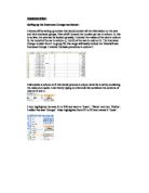
Below shows what the spreadsheet looks like once all the VLOOKUP functions have been entered.

                                

Column G produces the information in words and column H produces the multiplier figures.

Calculating the total cost of the quote.

The cost of the quote is calculated by multiplying together the numbers in column H.

I then set up a formula in cell H12 that would multiply together the figures in column H.

I set up a formula in cell H14 that would multiply the figure calculated in cell H12 by the no-claims percentage in cell F23.

Finally I set up a formula in cell H16 that would subtract the calculated figure in H14 from the calculated figure in cell H12.

Setting up the customer worksheet

I set up a separate worksheet that would file away and keep saved quotations. I set up the row headers like shown below.

Setting up the printout worksheet: 

I set up a new sheet and called it printed quote. Here I set up a page that would take the relevant information from the quote worksheet and could be used as a print out for customers and for the end user.

On the print out I have set a formula that will put today’s date on it, so that the date will be correct on each printout, and will not have to be done manually. I then typed in formulas that would copy the customer’s title, name, address and phone number from the quotes worksheet and show up the relevant information on the printout worksheet.

I then set up formulas that would duplicate the customer’s make and model of car, age, sex, no-claims discount and type of insurance. I then set up a formula that copied the final quotation price from the quotes worksheet.

Customising the interface and adding final touches:

My original interface looked like this:

I have customised this interface to look like this using the drawing tools in Excel and the company logo:

     

---

Setting up a macro to automate the filling of the quotes into the customer:

First I recorded a macro like above, this time I called the macro save quote.

This macro takes along time to record as it involves copying each of the necessary cells form the quotes sheet, then pasting the cells onto the customer’s worksheet.

I did this by selecting the first black row on the customer’s worksheet, c licking insert, rows. I did

 this so every time a new quote is saved it will be

added in at the top, without replacing old quotes.

I then switched back to the Quotes  sheet by using the toolbar at the bottom of the screen.

I subsequently selected the relevant cell, clicking Edit Copy, then switching to the customers sheet, clicking the relevant cell and finally Edit, paste Special. I used ‘paste Special’

So only what appears in the cell is copied and not any formulas any formulas that may have been in the cell.

Once I copied and pasted all the cells so the headers were all completed, I stopped recording the macro by using the visual basic toolbar and clicking ‘stop recording’.

This illustration shows the customer worksheet, containing some filled in quotes suing the save quote macro:

Setting up macros to get around my system:

On the quotes worksheet, I set up macros, that would let the user access the groups worksheet, the multipliers worksheet, view saved quotes and a macro that will let the user print the quote off.

The process that I went through to setting up the macros is what follows:

(This is an example of the macro I produced for flicking to a different worksheet)

1) Start recoding a macro

2) Name it

3) Switch it to relevant worksheet

4) Stop recording.

For the users to print off my quotes sheet I had to set up macro that would print off the final quotation sheet. I did this by: stat recording macro, d to the worksheet, from menu clicked file, print, O.k. and finally switch back to the Quotes worksheet and stop recording.

Adding the Auto-open and Auto close macros:

I wanted sought my system to be exceptionally user friendly and professional looking. So I set up an auto-open macro that would remove the gridlines, sheet tabs, row and column headings and scroll bars, when the system opened.

I set this macro by start recording, clicking tools, then Options, uncheck the gridlines, sheet tabs, scroll bars and row column headers. Uncheck the formula bar and status bar. Clicking view, toolbar and remove the Standard and formatting toolbar. Stop recording.

Also to make the system look professional as possible, I changed the header at the top of the system.

I used the Visual Basic Editor to edit the Auto-open macro. I clicked:

        -Tools

        -Macro

        -Visual Basic Editor. I opened the macro Auto-open and inserted the line Application.Caption = “Cheshire’s Vauxhall Insurance.”

                                                

                                                 

I set up macro buttons to make it easier and quicker for the user to run the macros. I did this by selecting the button icon on the forms Toolbar at the bottom of the screen and then drawing the button on at an appropriate point on the worksheet. A Menu appeared once I completed this, and I then assigned one of my macros to that button. In this case Iam producing a button that will let the user switch to the groups worksheet.

I then clicked on that macro and pressed o.k.

                I then right clicked on my macro button

and clicked edit text. I named the buttons suitable manes, like “View Quotes.”

Adding the User form:

To add the user form to my system I loaded Visual

Basic Editor by clicking Macro on the tools menus.

 I then clicked on Insert and User from and blank form appeared.

By using the toolbox I designed my User form. I set up the same header that I used on the printout sheet. I did this by clicking on label and drawing out a label at the top of the User from and typing out the heading.

I then added two command buttons that let the user Enter or Exit my system. I did this by clicking on the command button and drawing out a command button onto the page.

Validation:

The use of validation rules in my system was potentially to reduce the number of mistakes made for the user when typing in their information.

Firstly I added validation rules to the customer’s title by selecting the title cell and clicking Data on the toolbar and selecting validation.

I then chose from the list opposite what I would allow for that box, and then I pressed O.K.

This box then appeared, when ever the title cell was actively selected. (Below)

Secondly I added a validation rule to the customer’s forename and surname. I did this using the same process, which was selecting the relevant cells and clicking Data, then Validation.

I chose the text length to be between 1

 and 15 so errors such as holding downwards a key by mistake or missing the cells out which would result in an error.

        

I then typed in the error alert that would appear if the user typed in a word over 15 or left the cell blank.

I added validation rules also to the Customer’s addresses by adding a presence check, so an error message would appear if the cell were left blank. I did this by following the steps I did above for the other validation rules.

I added a validation rule also for the customer’s postcode; I did this by clicking Data and then Validation.

I then set the criteria to text length seven,

which would only allow the seven characters

needed for a postcode. I then typed in the

 message and then the error alert.

Finally I added a validation rule to the customer’s telephone number box, by clicking Data and Validation again. I set the criteria to be ‘equal to’ 12, which would allow all telephone numbers to be entered, from a mobile phone number to a different regional number from a different part of the UK.