In this experiment we will compare the internal resistance of the cells using required apparatus mentioned below. Thus internal resistances and other conductor components give a total resistance to the current of electricity in a circuit. We will be able to deduce the EMF of each cell.
Apparatus
- 2 large dry cells (one new and one old 1.5 volts)
- Rheostat
- Voltmeter 0-5 or 0-3 V)
- Ammeter (0-500mA)
- Switch
- Connecting wires
- Graph paper
Independent variables:
The currents (amps) is independent because we control/ adjusting it from the rheostat
Dependent variables
The voltage is gained after adjusting the currents from the rheostat that is why we called it dependent variable in this case.
Methodology:
1) Combination of cells
Firstly we measured the terminal p.d (potential difference) of each cell with a voltmeter. The red terminal of the voltmeter where connected to the more positive side of the cell. And then predicted the voltage we would measured for each of the following combinations shown below:
Measured each cell combination and then compare the prediction for each cell combination
Identified which combination would be used if you wanted an EMF larger than that from a single cell
Identified which combination is intended when cells are said to be “in series” and which intended when they are “in parallel”.
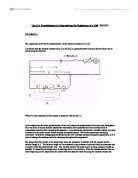
2) Set up the circuit shown in the following diagrams. Start for the rheostat set for maximum resistance. Picture shown below:
From a to b (see diagram)
-
There was a voltage gain of ε, the EMF of the cell.
- There was a voltage drop of Ir ( V = IR from ohm’s law)
So the combined potential difference measured on the voltmeter was:
V = ε – Ir where I is the current
3) Constructed the table showing how V varied with I (the value of I changed by adjusting the position on the rheostat)
4) Graphing the results gained after the experiment of new and old battery
5) Identified the gradient and the y- intercept of the best fit line for each set of the data
And for the values of the currents (independent variables) of both the old and new battery range from 0.0 to 0.6 amps in the old battery but in new battery also range from 0.0 to 1.2 amps
The Prediction’s results of the voltage and the combinations
The above table shows the prediction made before the actual measurement started off, so the best
combination we chose was in letter ‘b’ because the value of the emf is increasing compared to a single cell as well as its voltages increasing the most when the two cells combined
Identification for the combination of cells
Series combination Parallel combination
(b) (C) (C)
(C)
The results of the old and new battery
The old battery
Voltage and the currents
The New battery
The voltage and the currents
The two tables above resulted after the currents from the rheostat adjusted so the voltage depended upon the currents, it was given us a glue that when the currents from the rheostat increased the voltage getting decreased
Graphing the results of the two cells (old and new)
The above graphs were deriving from the previous table; it showed the emf and the internal resistances of the two batteries together. The upper most graphs were the new cell while the old cell held the lower part of the grid.
Calculation page for the old cell:
Old battery
A) Coordinate of the best fit line:
= (0.00, 1.31) and (0.60, 0.62)
Slope = internal resistance (-r)
Thus the internal resistance is -1.15 Ω
B) Coordinate of the error line: Hint: Y = mx + c since and r and Є are both constants
= (0.00, 1.35) and (0.6, 0.55) so: -r is the gradient of the graph (m)
Є is the intercept of the graph (c)
Slope of the error line is -1.33 Ω
C) Gradient uncertainty = Best fit gradient – error line gradient
-1.15 - -1.33
-1.15 + 1.33 = 0.18
Gradient uncertainty
D) y- Intercept = emf of the battery
y = mx + c or V = є - Ir
1.31 = є – (0.0) (-1.15)
є = 1.31volts
Calculation for the new cell:
A) Best fit coordinates
(0.0, 1.54) and (1.2, 0.98)
Slope = internal resistance (-r)
Thus the internal resistance is -0.49 Ω Hint: Y = mx + c since and r and Є are both constants
so: -r is the gradient of the graph (m)
B) Coordinate of the error line Є is the intercept of the graph (c)
(0.0, 1.55) and (1.2, 0.96)
Slope of the error line is -0.49 Ω
C) Gradient uncertainty = Best fit gradient – error line gradient
= -0.47- - 0.49
= -0.47 + 0.49 = 0.025
Gradient uncertainty = 0.47 ± 0.025 Ω
D) y- Intercept = emf of the battery
y = mx + c or V = є - Ir
1.54 = - (0.46) (0.0) + є
є = 1.54 volts
Discussion:
Table one;
The result from table one of an old battery, occupied small readings (intervals) of the currents of 0.1 amps together with the value of uncertainty of ± 0.1, and these values altered the value of the voltage. According to the graph of table one the origin of the line graph faced towards the negative side thus the slope of the linear graph is – 1.15 and the y-intercept of 1.31. The internal resistance of the old battery obtained from the linear graph, so the gradient of the line is the internal resistance of the old battery that is 1.15Ω (ohms) and the y-intercept represented the EMF of the cell ε that is 1.31 V
Table two:
In the result of table two (new battery) the readings of the currents is adjusted from the rheostat where it affects the values of the voltages. The potential difference of the new battery is 1.5 volts, the values of the currents is adjusted using the interval of 0.01 amps and last at 0.06 amps. At 0.00 amps (currents) the volt meter reached 1.5 volts and when 0.06 amps the voltages was 1.03 the value of the uncertainty we used ± 0.01 after obtaining all the voltages from the currents readings we came with the gradient of – 0.4 through the y- intercept of 1.54 amps ( x- axis). The graph was clearly displaying the results of the adjusting currents to the voltages together with the y- axis and the slope line thus the EMF of the cell ε is 1.54 V ( y- intercept) and the internal resistance of the cell is should be in negative gradient of – 0.4 Ω (G.Alex)
Moreover according to the formula given in the procedure V = є –Ir we used it to identify the
emf (potential difference of the battery before connected to the circuit) by rearranging the above formula
to make є the subject, then substituting the value of V (the voltage of both old and new battery), the current and the internal resistance then multiplied the value of I with the internal resistance r and later subtracted it with the value of V in order to obtain the emf (the potential difference of the cell), this formula helped to calculate or to proof the variable of the unknown above symbols especially the emf.
During the practical experiments, we were not sure yet about our results whether are true or not but after the research it satisfied us with an idea that the voltage of the each cell is inversely proportional to the currents in this case. It meant that our experimental results were similar with theories and other prior experimental results thus indicating that the voltage should inversely proportional to the currents.
From the results different readings (from the old and new) of the potential difference of the battery, this relied on the strength of the battery the stronger the battery the more reading required. So on the graph the upper linear is the resultant of the new battery while the lower one indicated the old battery because it had a lower emf (potential difference) because it had been using up. The trend of the graph showed that the older cell was steeper than the new cell, main reason for this trend stated that when the cell getting old the internal resistance started to built up so less of the voltage driven from the battery
Conclusion:
For the overall results, there were slight differences in the emf and the internal resistances between the two batteries this depended upon the use of time, so from the experimental parts and after the calculations I could find that the emf of the old cell was less than the emf of the new cell. The internal resistance found greater in the old cell and less in the new cell, as the cell getting old the resistance inside accumulated because of the expired time of the chemicals,
The best combination we found after the practical experiments was in letter ‘b’ connected in series as it doubled the voltage of each cell.
The value of the emf of the new cell was 1.54 volts with it internal resistance of -0.49 Ω and the value of the emf of the old cell was 1.31volts with it internal resistance of -1.15 Ω
So it looks like this; at first the new cell rich in potential differences but after time, the internal resistance getting built up that means it becomes outlive it potential differences (flat) and then becomes as one of the old cell because it emf is less than before and the internal resistance is increasing
Bibliography:
- P.Howison, 1999,Physics year 13, ESA Publications (NZ) Ltd, Singapore
- Encarta 2006, Internal Resistance, Microsoft Corporation
- Britannica 2006, Internal Resistances, Britannica Corporation
- G.Alex, 23 May, Internal resistances, www. battery.com,
Appendix: 1
The set up photo of the practical using the old cell
The above picture shows the components of the cell together with the lighting bulb
The set up appratus for the new cell