a = v2 / 2s
Hence, it was possible to find the acceleration along the slope by taking the gradient of the resulting regression lines plotted through the data. This could then be used to find the acceleration due to gravity. However, due to the number of possible sources of error, a perfectly accurate result would be tricky to obtain.
The resulting graph is found in ‘Appendix 1 – Graph of results’. From this, the gradients of the regression lines through the data were taken. These are shown below;
When Ɵ = 10.8˚, a = 1.6373 ms-2
When Ɵ = 6.6˚, a = 0.7338 ms-2
When Ɵ = 3.3˚, a = 0.3367 ms-2
Therefore, if we know sin Ɵ and a, it is possible to estimate g - the acceleration due to gravity.
For each value of a, to calculate g, we apply the formula;
g = a / sin Ɵ
This gives us 3 values of g, calculate purely without taking friction and other error into account;
When Ɵ = 10.8˚, a = 1.6373 ms-2, sin Ɵ = 0.187 (3s.f.), hence g = 8.756ms-2 (3d.p.)
When Ɵ = 6.6˚, a = 0.7338 ms-2, sin Ɵ = 0.115 (3s.f.), hence g = 6.381ms-2 (3d.p.)
When Ɵ = 3.3˚, a = 0.3367 ms-2, sin Ɵ = 0.0576 (3s.f.), hence g = 5.845ms-2 (3d.p.)
These values prove the theory that friction has less of an impact at higher angles. It is evident from the results that, as the value of Ɵ increase, as does the calculated value for g. The values obtained clearly show the presence of error as the calculated values for g in this experiment differ from the widely accepted value of g; 9.81ms-2. Because we already know that friction has a smaller impact on the results at higher values of Ɵ, this alone could explain the error and trends shown in the values for g. However, it is very unlikely to be the only source of error in the experiment.
In the following section, errors will be discussed and a new value of g will be calculated, this time taking friction into account. While this provides a more suitable value for g, the error that is incorporated into the result as a consequence makes the new calculated value of g a lot less reliable.
Error
Certainly, the experimental setup contained many errors, some systematic, some random. The following section discusses what was done to detect and correct systematic errors and outlines the key random errors and suggests how these impact the results.
Undoubtedly, there was random error in the data. Possibly the most important piece of random error to consider is the starting velocity not being 0. While it was attempted that trolley was released without accidentally pushing it, there may have been circumstances where the initial velocity wasn’t 0, meaning that the final velocity would have been higher than expected. This error can be partly compensated for by adding error bars to the graph, which incorporate values of v2 which may be higher than measured. The problem of the error is exaggerated by the fact that v2 is exactly that; squared. This means that any error incorporated into that figure is also squared, leading to further inaccuracies. Furthermore, because the trolley is accelerating down the ramp, the velocity is increasing exponentially, meaning small inaccuracies of the initial velocity can have a big different on the final velocity. However without any method of knowing whether the initial velocity was 0, the only thing to do is add error bars that may or may not cover this error. In order to find errors bars of a suitable size, it was necessary to find the maximum deviation from the mean for each data point in each data set. Then, for each data set, the maximum deviation used a ± figure for the size of the error bar. For example, with the ramp at 6.6˚, the maximum deviation was -0.087053078, hence the error bars ‘width’ for that data set was set to ±0.08705. If the experiment was repeated, the trolley could be held initially with an electromagnet which could then be turned off. This would ensure that the initial velocity was 0, or certainly, negligible.
A further random error was introduced into the results by the accuracy of the 5mm LEDs on which the light gates work. Between the ‘gate’ of the light gate, there are two IR LEDs, which maintain a beam between them. Simply put, when the beam is broken, this sends a signal to the main processor, which starts the timing. The signal from the LED which is detecting the IR radiation sends its signal when the intensity of IR reaching it reaches a certain point. Without doing a complicated experiment, there is no way to determine at what level or intensity of IR the light gate will start or stop timing. Furthermore, because the experiment was done in a room which was lit by natural light (in this case, the main source of IR), the background intensity of IR will have fluctuated from each result. This means that for each time the card passed through the light gate, timing could have started at a different point. While this difference would be minute, the value is used to calculate v2, and hence any error which the calculation of v incorporates is squared, and made more significant. To further improve accuracy of the results, it would be necessary to do the experiment again in a place that suffers from less IR light pollution.
Another factor which contributes to the uncertainty associated with light gate is the position of the emitter and receiver within the LED and furthermore, the position of the LED. The distance measured from the starting point and where the beam actually is in the light gate could differ by a few millimetres. This could be due to the position of the LEDs within the gate or the point at which the beam is ‘fired’. This is better shown in the diagram below (fig. 4). While it is hard to find out where the actual point of the source of the LED, it is possible to measure to the centre of the LED and from here add a ± value equal to the width of the LED. Since the LEDs are 5mm wide, this becomes ±2.5mm. This ±2.5mm has a greater percentage error at distances closer to the light gate than distances further from the light gate. In order to incorporate this percentage error into the final percentage error, it is necessary to take the maximum possible percentage error;
(2.5 / 350) x 100 = 0.71% (2d.p.)
Figure 4 – A diagram showing possible places from which the beam could begin. The arrows show possible places where the emitter could be, and the red LED and corresponding red arrows show an alternative position of the LED.
Two further systematic errors that can be easily accounted for are the length of the card and the trolley accelerating through the light gate. Because the light gate was calibrated to calculate the velocity using a distance of 100mm (the apparent length of the card), if the card was not actually 100mm, this would induce a systematic error in the calculated velocities. In order to account for this, the time measured was used, which was ‘raw’ data, i.e. it hadn’t been processed through a formula. The piece of card was measured using vernier calipers to give a value of 102.0mm ± 0.5mm (the tolerance of the calipers). This was then used in conjunction with the time that was measured to calculate the velocity according to the formula;
velocity = displacement / time
The percentage error relating to the measurement of the piece of card can also be incorporated into the final percentage error. This is calculated in the following way;
(0.5 / 102.0) x 100 = 0.49% (2d.p.)
It is important to consider that although the distance from the front of the card to the centre of the light gate was, for example, 250mm ± 3.0mm, the trolley is actually accelerating all the way through the light gate. Therefore, it is actually accelerating for a distance equal to the distance from the marker to the middle of the LED plus the length of the card being used. In the case of the measurement of 250mm ± 3.0mm;
Actual distance that the trolley is accelerating for = 250mm + 102mm = 352mm.
As for the percentage error that accompanies this distance of 352mm, it is simply the percentage error of the measurement of 250mm added to the percentage error of the measurement of 102mm;
1.2%+ 0.49% = 1.69%
Thus, it is possible to calculate the 1.69% as a distance;
(352 x 1.0169) – 352 = 5.9488mm
Hence the actual distance that the trolley is accelerating for is 352mm ± 5.9488mm
Therefore, it is important to scale the value of 2s so that it is equal to twice the distance that the trolley was accelerating for, rather than it being twice the distance between the front edge of the card when the trolley was at rest and the centre of the light gate. This involves adding 102mm to every value of s, which has been done, as seen in the data table.
Another possible random error could be induced by the card not going through straight. Indeed, while doing the experiment, some values did seem to be obvious outliers and the cause of this, when examined, was that the card was not going through perpendicular to the light gate. These were then re-done and the previous value discarded. It was also appropriate to check that the card was parallel to the plane and perpendicular to the light gate, or else systematic error would be induced. These checks were made beforehand using a set square and the equipment was altered if the results from these checks did not meet the conditions. If the card was even slightly skewed, this could have a significant impact on the results, as shown below in fig. 5.
Figure 5 – A diagram showing the distances measured when the card is on a tilt.
Clearly from the diagram, it is possible to see that with the card at any angle which isn’t perpendicular to the light gate, the time taken for the card to pass through the light gate is different. However, without any knowledge of if the card was on a tilt or not for any values, it is impossible to calculate the new length of the card. If the experiment was to be repeated, attempting for maximum accuracy, the card would be clamped or screwed to the trolley, reducing the possibility that it could come loose.
A critical piece of systematic error was that the desk on which the experiment was done wasn’t flat. In fact, the whole desk was on a consistent slope of -0.5˚±0.1, which was the same down five places at different intervals down the desk. Arguably, while this figure carries a 20% percentage error, the fact that five measurements were taken and the value was the same all the way along improves the precision of the results. Despite this, there was no other way to successfully measure the slope of the desk; hence this value had to be used. In order to account for this systematic error, the value of -0.5 was added to every value of Ɵ obtained by trigonometry, effectively making the results reflect what they would have been if they had been taken if the desk was flat.
When measuring the angle of the ramp, it was more appropriate to use trigonometry than a digital spirit level. This was because the digital spirit level could only measure to ±0.1˚, whereas using trigonometry could theoretically calculate the angle to a large number of decimal places. However, this does rely on measuring the distance between the centre of the light gate and point up the ramp and vertical heights to be exactly right. Despite this, the percentage error of measuring the angle of the ramp using trigonometry works out less than measuring with a digital spirit level;
For an angle of 10.8˚;
On a digital spirit level; angle = 10.8˚ ± 0.1˚. Thus, the percentage error is 0.93% (2d.p.)
However using trigonometry;
It is possible to use the sine rule to calculate the missing angle Ɵ;
a / Sin A = b / Sin B = c / Sin C
1750 / Sin 90 = 374 / Sin Ɵ
Because Sin 90 = 1;
1750 / 1 = 1750
Thus; 374 / Sin Ɵ = 1750
Therefore;
374 / 1750 = Sin Ɵ = 0.214 (3d.p.)
Sin-1 0.214 = 10.836˚
It is acceptable to say quote that the value of 374mm lies within ± 0.5mm due to the use of set squares to ensure that the measurements were taken at 90˚ to the plane (the desk). This made the measurements very precise and accurate. Since the percentage error will be significantly greater in the measurement of 374mm than the measurement of 1750mm, it is acceptable to use just this percentage error as the final percentage error for the two measurements;
0.5 / 374 x 100 = 0.14% (2d.p.), giving the value of 10.836˚ a percentage error that is 5 times smaller than that of the same measurement using the digital spirit level.
There was almost certainly other systematic and random errors in the experiment, however, once considered, these were largely reasoned to be counted as negligible. Such errors would be the tolerance of the reading of the time on the light gate. This was ±0.005ms, hence for the minimum value of time recorded (42.73ms), the percentage error was only 0.000117%. Other errors included in this category of negligible would be; temperature of the room causing expansion of all equipment used, especially in measuring equipment such as rulers; air currents in the room causing air resistance or following wind to have an accelerating or decelerating effect on the movement of the trolley; and residue or substances on the ramp or wheels of the trolley causing an increase in the friction of the trolley.
Finally, another systematic error could have been introduced when the distance from the light gate were measured. Since the light gate had to be suspended in the air, it was hard to fix it such that the light gate was perfectly perpendicular to the ramp. Due to the mechanism of the clamp, it was extremely difficult to get the light gate to stay perpendicular to the ramp. This induces an error similar to the one induced if the card was not perpendicular to the light gate. If both were present, they could theoretically cancel each other; however it is also possible that they could have both contributed. In order to attach a percentage error to the angle at which the light gate was in comparison to the angle of the ramp, it was necessary to measure the angle of the light gate. Since this could only be done with a digital spirit level, the final percentage error contains both the tolerance of this device and the compared value of the angle of the light gate to the angle of the ramp. In order to completely account for all the possible data errors, it is necessary to use the distance and angles at which the most error was present. To calculate this, 3 measurements of the angle of the light gate were taken; one for each value of Ɵ;
Angle of the light gate when Ɵ = 3.3˚; 3.1˚ ±0.1˚
Angle of the light gate when Ɵ = 6.6˚; 6.0˚ ±0.1˚
Angle of the light gate when Ɵ = 10.8˚; 10.5˚ ±0.1˚
Thus, from the above data, we can see that the most error for the angle of the light gate was when the ramp was at 6.6˚. Also, it is possible to see that the most error induced by the tolerance of the digital spirit level was when Ɵ = 3.3˚.
Using this information, we can now calculate the percentage error associated with these measurements;
Error induced by the differing angles of the light gate and the ramp;
(0.6 / 6.6) x 100 = 9.09%
Error induced by the tolerance of the digital spirit level;
(0.1 / 3.1) x 100 = 3.23%
Using all the percentage errors calculated from systematic errors, it is possible to add all these together to give a final error which can be then applied to each measure of g;
Error induced by the differing angles of the light gate and the ramp: 9.09%
Error induced by the tolerance of the digital spirit level: 3.23%
Error induced by inaccuracies in measurement of the distance: 0.14%
Error induced by the equipment used to measure the piece of card: 0.49%
Error induced by measuring the distances along the ramp and LEDs: 1.20%
Thus, total error: 14.15%
This value of the error can then be converted into an actual figure for each value of g produced;
When Ɵ = 10.8˚, g = 8.756 (3d.p.)
8.756 x 1.1415 = 9.994974
9.994974 – 8.756 = 1.238974
Hence when Ɵ = 10.8˚, g = 8.756ms-2 ± 1.238974
This can then be done for all other calculated values of g;
When Ɵ = 6.6˚, g = 6.381ms-2 ± 0.902912
When Ɵ = 3.3˚, g = 5.845ms-2 ± 0.827068
While the above data provides a good estimate for g, it does not take friction into account. This is certainly the greatest systematic error. In order to find a value for the friction and hence calculate a much more accurate result for the value of acceleration due to gravity, it was necessary to set up a further experiment as described at the end of the ‘Theory’ section, the aim of which was to find out at what angle the friction balanced the angle of the slope, i.e. when Fr was equal to mg sin Ɵ. At this point, the trolley would be stationary. The result of this experiment was that the angle that balanced the effect of friction was 1.7˚±0.1, due to the tolerance of the electronic spirit level used.
This value was obtained by measuring the angle of the ramp at three different positions and taking an average of the angle of the ramp. This was necessary to do because the ramp was slightly bent i.e. it ‘sagged’ in the middle. The three measurements taken had a range of 0.4˚, giving the angle of the friction compensated ramp a final uncertainty value of 1.7˚± 0.5˚. Since μ = tan Ɵ, in order to convert the error for the angle to an error for μ, it was necessary to change the ±0.5˚ into a percentage. This was done by the following calculation;
(0.5 / 1.7) x 100 = 29.41% (2d.p.)
Therefore, tan Ɵ = μ = 0.029679 (5s.f.) ±29.41%
Hence, μ = 0.029679 ±0.008729
This error becomes very significant when calculating g. If, for example, we take the data from when Ɵ = 3.3˚;
g = a / (sin Ɵ – μ cos Ɵ)
Using the maximum possible value of μ (0.029679 + 0.008729);
g = 0.3367 / (sin 3.3 – (0.038408 x cos 3.3)) = 17.518 (3d.p.)
However using the minimum possible value of μ (0.029679 - 0.008729);
g = 0.3367 / (sin 3.3 – (0.02095 x cos 3.3)) = 9.187 (3d.p.)
This shows that the small inaccuracy in the measurement of the angle of the ramp that equates Fr can have a massive impact on the final result for g.
However, at larger values of Ɵ, i.e., when the ramp was steeper, this error becomes less. This is because the percentage error that the value of μ contributes to the overall percentage error is much less than when Ɵ is smaller. This is better shown mathematically;
Using the maximum possible value of μ (0.029679 + 0.008729), and the angle of the ramp being 10.8˚;
g = 1.6373 / (sin 10.8 – (0.038408 x cos 10.8)) = 10.941 (3d.p.)
However using the minimum possible value of μ (0.029679 - 0.008729);
g = 1.6373 / (sin 10.8 – (0.02095 x cos 10.8)) = 9.816 (3d.p.)
Obviously then, at smaller angles, the percentage uncertainty is much larger. Therefore it is also appropriate to say that at larger angles, the percentage uncertainty is lower. This comes down to the fact that sin 10.8 > sin 3.3. While this seems obvious, as shown in the previous calculations, it has massive implications. Because sin 3.3 is a comparatively small number, when μ cos Ɵ is subtracted, this makes the resulting value very small;
sin 3.3 – μ cos Ɵ = 0.05756 – (0.029679 x cos 3.3) = 0.02793 (5d.p.)
Thus, when this number is divided by a, the acceleration down the slope, the result is comparatively large;
0.3367 / 0.02793 = 12.055 (5s.f.)
However, small variations in the value of sin 3.3 – μ cos Ɵ have a large implication on the outcome. For example, if sin 3.3 – μ cos Ɵ = 0.025, then;
g = 0.3367 / 0.025 = 13.468 (5s.f.)
This is a change of nearly a 1 and a half metres per second per second from a slight change in the value of sin 3.3 – μ cos Ɵ.
However, at larger values of Ɵ, which occur when the ramp is steeper, the value of sin Ɵ – μ cos Ɵ becomes larger;
sin 10.8 – μ cos Ɵ = 0.18738 – (0.029679 x cos 10.8) = 0.15823 (5d.p.)
The means that uncertainty of the value of μ has less of an impact on the results. This is due to the values being nearly of the same magnitude;
Angle of ramp: 10.8 Angle of ramp: 3.3
Value of sin Ɵ – μ cos Ɵ = 0.15823 Value of sin Ɵ – μ cos Ɵ = 0.02793
Value of a = 1.6373 Value of a = 0.3367
sin Ɵ – μ cos Ɵ as a percentage of a: sin Ɵ – μ cos Ɵ as a percentage of a:
(0.15823 / 1.6373) x 100 = 9.66% (0.02793 / 0.3367) x 100 = 8.29%
From the above table, we can see that when the angle of the ramp is at 10.8˚, ‘sin Ɵ – μ cos Ɵ as a percentage of a’ has a higher value than when the ramp is at an angle of 3.3˚. This information demonstrates that the higher value of sin Ɵ – μ cos Ɵ for the ramp at 3.3˚ induces more error because the values for a and sin Ɵ – μ cos Ɵ are further apart in terms of magnitude than the same values for when the ramp is at 10.8˚. Despite the inaccuracies that become included when friction is taken into account, these values are more precise values for g than those which were calculated without taking friction into account. For these new values, the error is the same as before, with the added error for the calculation of μ;
14.15% + 29.41% = 43.56%
Hence, the new values of g can be calculated, this time taking friction into account, and the percentage error of 43.56% can be converted into an actual amount;
To calculate g, we use the formula;
g = a / (sin Ɵ – μ cos Ɵ)
So for when Ɵ = 10.8˚;
g = 1.6373 / (0.18738 – (0.02793 x 0.98229)) = 10.237ms-2 (5s.f.)
A similar calculation can be done for the other values of Ɵ;
When Ɵ = 6.6˚;
g = 0.7338 / (0.11494 – (0.02793 x 0.99337)) = 8.416ms-2
And for when Ɵ = 3.3˚;
g = 0.3367 / (0.05756 – (0.02793 x 0.99834)) = 11.346ms-2
Finally, it is necessary to change the percentage error of 43.56% into a value for each result;
When Ɵ = 10.8˚; g = 10.237ms-2 ±43.56% = 10.237 ms-2 ±4.459
When Ɵ = 6.6˚; g = 8.416ms-2 ± 43.56% = 8.416 ms-2 ± 3.666
When Ɵ = 3.3˚; g = 11.346ms-2 ± 43.56% = 11.346 ms-2 ± 4.942
While these percentage errors seem rather high, these are maximum values. It is more likely that some measurements will have been under-measured and others over-measured, hence the actual percentage error which would be found in any one setup would likely to be less than this theoretical value. It is also evident from results that the known value of 9.81 lies somewhere within the upper and lower bounds of each result.
Conclusion and evaluation
From the results, it was possible to draw 3 values for g; one for each angle of Ɵ. With the largest sources of error considered, it was possible to add a percentage uncertainty value to each of these results. From here, it was possible to convert each of these percentages into an actual uncertainty. While this may have appeared to have been a lot, there was a lot of error in the experimental setup, despite best efforts to reduce systematic error. However, while the results were questionable in accuracy, they were precise, with 9.81 lying somewhere within the upper and lower bounds of each value.
If the experiment was to be repeated, the following things would be changed. All of these aim to further reduce error which could be only be accounted for in the write up, rather than in experimental practice.
- The trolley would be held in place with an electromagnet which could be remotely turned off so as to remove the possible random error of the initial velocity not being equal to 0.
- The light gate would be attached to the ramp, so as to make sure the two pieces of equipment were perfectly perpendicular. this would reduce the error induced by the light gate measuring a distance that is more than the actual length of the card.
- The piece of card would be screwed or held firmer in place in the slot in which it was supposed to be held. This would reduce the chance of the card being skewed as it passed through the light gate.
- More accurate measuring equipment (mainly rulers) would be used to reduce the systematic errors contributed when key measurements were being taken.
- The experiment would be done under controlled environmental conditions; the amount of IR radiation falling onto the apparatus would be kept constant.. This would keep the response time of the light gate consistent.
- More values for the measurement of the angle at which friction balanced the acceleration would be taken, leading to a more accurate result for μ, which, in this experiment, was the biggest contributor of error.
- A ramp that was perfectly flat would be used; this would reduce the chance that bowing of the wood could induce possible error into the values for acceleration.
If most of these improvements were made, the expected result would be that the values of g would become more precise, with less uncertainty associated to them.
Investigating the forces on a trolley down a ramp