Investigation about the spring loaded plunger
Figure 4. Finding spring constant experimental set up
Experimental Set up: Fixed the trolley using a clamp and at the same time fix a ruler next to it, then Measure the original length of the spring.
Method: place 50g of mass on the spring increasingly. Record the corresponding length of the spring and calculate the compression of the spring every 50g. From this we can find out the spring constant k in formula F = -kx.
Table 1: Spring constant – Force vs. Compression
Corresponding error is ±0.001
Graph1. Spring constant – Force vs. Compression
The gradient of this spring is 0.0026 where
To find the velocity, we know that the area under the graph is energy stored in spring with conservation of energy, the energy stored is turned into Kinetic energy but this is when assuming there is no air resistance or any other kind of energy lost.
Figure 5.- a spring loaded plunger
There are three different set of forces in a spring loaded plunger and I am going to use the first two sets of force where the compression is 3cm and the other 6 cm; and will label them as “small force”, “big force” respectively.
From theory, with the compression length above to shoot a table tennis ball, we found that:
For a small force, the theoretical velocity is as below:
v= 12 ms-1 (2.s.f)
For a small force, the average experimental velocity= 6.5 ms-1
For a big force: (2.6g= 0.0026kg)
v=23 ms-1 (2.s.f)
For a big force, the average experimental velocity= 11.5 ms-1
Then I am going to calculate the velocity of a squash ball with the use of a big force. (This is for further use in the experiment).
In both “big” & “small” force experiments, the recorded speed is halved compare with the experimental value. Since, only of elastic potential energy is change to kinetic energy of the table tennis ball. It indicates the work done against air resistance is significant (on the table tennis), so I am going to work on squash ball afterwards.
The following are the theoretical and experimental value of a squash ball with a big force:
Same equation with a different mass of 0.024kg = 24.1g
v= 7.6 ms-1 (2.s.f)
For a big force and a squash ball, the average experimental velocity= 3.5 ms-1
Air resistance is only a small factor that affects the velocity of the ball. The main reason is that in the calculation, I have assumed that energy is conserved, however, that is not true in practical work. Some energy is lost in work done in spring, lost to the surrounding as heat and not all the Elastic Potential Energy in spring is transferred to the ball as K.E, then some K.E goes to the mass at the end of the spring. The main thing is that the spring do not bounced back to the original length when the ball is released therefore not all force is transferred to the ball. Therefore all I can conclude is that the spring has 50% efficiency.
Precautions/ Safety:
Before the experiment, I handed in a plan and was approved at a safety angle by teacher. During the experiment I have also considered many aspects of safety issues. For example, making sure that when I shoot the ball with the spring loaded plunger, I would not hit anyone and the use of balls; making sure the ball is not hard to hurt anyone.
Error in Range and % error calculation
Error in range = (max range – minimum range)/2
% error calculation = Error in range / Average Range
The following graphs’ error bars are plotted using the average percentage error.
Preliminary Investigations
In this investigation, a table tennis ball is chosen for trials because it is very light and is able to be fired off to a long distance.
Method:
I shoot a table tennis ball towards a sand pit at different angles using a “small” force and measure the range of the ball when it first land using a tape measure. I then record the corresponding horizontal distance as the angle varies; where angle is measure using a protractor. (Apparatus set up based on Fig 3.- without light gate)
Prediction:
I expect that the optimum angle for maximum range will be around 40-50 degrees, according to the theoretical value 45 degrees I have calculated earlier.
Results:
Diameter of the table tennis ball: 29 mm Average weight of the ball: 2.6 g
Table2. Shooting a table tennis ball with a ‘small force’- (for experiment 1)
Average error in range= 0.05 = 5%
Graph 2: Angles vs. Horizontal Distance- (for experiment 1)
This is to find the optimum angle for shooting a table tennis ball with a ‘small average force’
Conclusion:
This preliminary experiment has shown that the ball can be fired properly and from my graph of results I can conclude that, there is an optimum point is 33±10 degree, however, I am not very certain and am not confident the optimum range within ±5 degree therefore would like to improve it to get a more accurate optimum angle.
Evaluation:
From this experiment, I have also learnt that because the table tennis ball is too light and the force given is very small, therefore it is strongly affected by air resistance which affects the range. The range need to more separated in order to get a more distinct set of results. This can be improved by increasing the force of the shot.
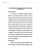
Figure 6. a picture of part of an experimental set up
Method:
I repeated the method used in the previous experiment but have I changed the strength of the ball to a “big” force and has added a light gate to my experiment so that the average force of the ball can be recorded and be compared to the theoretical value. (Apparatus set up based on Fig 3.)
Prediction:
I predict that it will give a longer range and gives a more distinctive optimum angle on the graph.
Results:
Table 3: Shooting a table tennis ball with a ‘bigger force’ - (for experiment 2)
Average error in range= 0.1 = 5%
Graph 3: Angles vs. Horizontal Distance - (for experiment 2)
This is to find the optimum angle for shooting a table tennis ball with a ‘bigger average force’
Conclusion:
According to the graph of results supports my prediction; a larger force gives a bigger range. However, my investigation did not produce a single distinct optimum angle. This is because air resistance increases with velocity which intern increase in force. (Detail referring to page 9). From this, I conclude that the optimum angle is 32±7 degree.
Evaluation:
To be more accurate and be more similar to a basketball since from the results above, air resistance will contribute an important part in my modeling. By eye and feelings, table tennis is too light and doesn’t have the same ratio as basketball and might not act like a basketball. Therefore, I am going to investigate the two important factors which affect air resistance- mass and cross sectional area of the ball.
Research about Basketball
Comparing a basketball to other sport balls with a similar shape and material
Figure 7- Mass weighing
Method:
Find the mass of the 3 balls, then the diameter of the balls using a ruler and a micrometer. Then calculate the cross sectional area using the equation S.A =πr2
Results:
Table 4
Cross-section area is one of the important factors that affect air resistance by working out that the “cross-section area to mass” ratio of the balls. From the table above, it shows that the squash ball will be the best model to a basketball comparing to a table tennis ball because its mass-to-cross-section area is much closer to the basketball comparing to the balls with a similar size (e.g. a table tennis ball and a squash ball). Experiment is now changed to squash ball.
Method:
I repeated the method used in the previous experiment but I have changed the ball from a table tennis ball into a squash ball. (Apparatus set up based on Fig 3.)
Prediction:
Smaller in range however since surface area is about the same, mass increases, velocity decreases therefore air resistance will decrease comparing to the previous experiment however should give a more distinct drop between the surrounding points and the maximum point.
Results:
Table5 – (for experiment 3)
Average error in range= 0.2 = 7%
Graph 4 (for experiment 3)
Conclusion:
By changing from a table tennis ball to a squash ball the corrolation of the graph is now 0.9904 which is much more accurate. I can confidently conlclude that the optimum angle of shooting from a higher level to the ground with a parabola path is 33±5 degrees.
Evaluation:
My results are more reliable than before and gives a more disticncted levels between points therefore I can predict more accurately for the optimum angle. Now I would like to start investigating whether height affects the optimum angle.
Method:
I repeated the method used in the previous experiment but I have increased the height of the sand pit (set up is shown on figure 9).
Table 6 - (for experiment 4)
Prediction:
As height increases, the optimum angle gets closer and closer to the theoretical optimum value of 45 degree.
Average error in range= 0.2 = 11%
Results:
Graph 5. - (for experiment 4)
Conclusion:
From the graph, I can confidently conclude that the optimum angle of this experiment is 35±5 degrees. The results from my graph intends to agree with my prediction; as height increases, the optimum angle gets closer and closer to the theoretical optimum value of 45 degree.
Evaluation:
However, two set of results does not verify the fact that it is the trend therefore to improve it; I am going to do another set of results with an increase in height of the sand pit.
Method:
I repeated the method used in the previous experiment but I have increased the height of the sand pit as the same level as the take off point of the runway. (The apparatus set up is shown on figure 9).
Prediction:
Refer to page 18 – prediction.
Results:
Table7- (for experiment 5)
Average error in range= 0.06 = 4%
Graph 6- (for experiment 5)
Conclusion:
From the graph, I can confidently conclude that the optimum angle of this experiment is 41±5 degrees. The results from my graph confirm that it agrees with my prediction; as height increases, the optimum angle gets closer and closer to the theoretical optimum value of 45 degree.
Conclusion
As the height of sand pit increases to level with launch, with a constant shooting point, the optimum angle increases and will be closer to the theoretical angle of 45 degree as it get to the same level as the shooting point.
From the results above, I can predict and expect that when the height of the sand pit is fixed (a basketball ring- in real life), the optimum angle for a lower shooting point (short person) will be further from the optimum angle than from a higher shooting point (a taller person).
Evaluation
Although my experiments proved the trend between height and optimum angles, there are lots of other ways to further investigate and improve my investigation.
There are errors in measurements
-
Apparatus error e.g. the accuracy of protractor and ruler for measurements is ±0.5 cm and ±0.5 degree respectively.
- Inconsistency of the force when shooting using a spring loaded plunger
To improve my investigation, I can firstly use more accurate apparatus. Then have a better and wider range of results with a smaller interval between results.
For further investigations, I then find out the relationship between different types of balls and different speed of balls and see how they affect the optimum angle of a shot.
Sources
-
(reference for definition)- page1
- Advanced Physics (p.118) by Tom Duncan
- Mechanics 2 by John Hebborn and Jean Littlewood
- facstaff.gpc.edu/~ulahaise/The%20Physics%20of%20Basketball.ppt