Area in the right tail = α = .05
The degrees of freedom are calculated as follows:
k = number of categories = 3
df = k −1 = 3 − 1 = 2
From the Chi-square distribution table, the critical value of χ2 for df = 2 and .05 area in the right tail of the chi-square distribution curve is 5.99
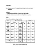
As the value for p is 0.45 and the value for q is 0.55 with a total sample of 20 individuals, the expected genotype frequency of p2 = AA = 0.2025
Expected number of AA individual= expected genotype frequency of AA x Sample
= 0.2025 x 20 = 4.05
Expected genotype frequency of Aa = 2pq = 0.495
Expected no. of Aa individuals = Expected genotype frequency of AA × Sample
= 0.48 × 20 = 9.90
Expected genotype frequency of aa = q2 = 0.3025
Expected no. of aa individuals = Expected genotype frequency of aa × Sample
= 0.3025 × 20 = 6.05
Table 3: Chi-square test for parental (P) generation
Hence the calculated value of X2 = 0.90 is smaller than the critical value of 5.99. Therefore we accept the null hypothesis and state that the dominant and recessive alleles of the parental generation of this sample and conform to the Hardy-Weinberg equilibrium of genotypes.
Chi-square test for the F5 generation
The hypothesis:
H0: The dominant and recessive alleles of the parental generation of this sample conform to the Hardy-Weinberg equilibrium of genotypes.
H1: The dominant and recessive alleles of the parental generation of this sample do not conform to the Hardy-Weinberg equilibrium of genotypes.
At the 5 % significance level, we already know that the Chi-square test is always right-tailed. Therefore, the area in the right tail of the Chi-square distribution curve is,
Area in the right tail = α = .05
The degrees of freedom are calculated as follows:
k = number of categories = 3
df = k −1 = 3 − 1 = 2
From the Chi-square distribution table, the critical value of χ2 for df = 2 and .05 area in the right tail of the chi-square distribution curve is 5.99
As the value for p is 0.45 and the value for q is 0.55 with a total sample of 20 individuals, the expected genotype frequency of p2 = AA = 0.1225
Expected number of AA individual= expected genotype frequency of AA x Sample
= 0.5625 x 20 = 2.45
Expected genotype frequency of Aa = 2pq = 0.455
Expected no. of Aa individuals = Expected genotype frequency of AA × Sample
= 0.455 × 20 = 9.10
Expected genotype frequency of aa = q2 = 0.4225
Expected no. of aa individuals = Expected genotype frequency of aa × Sample
= 0.4225 × 20 = 8.45
Table 4: Chi-square test for the fifth (F5) generation
Hence the calculated value of X2 = 2.32 is smaller than the critical value of 5.99. Therefore we accept the null hypothesis and state that the dominant and recessive alleles of the parental generation of this sample and subsequent generation conform to the Hardy-Weinberg equilibrium of genotypes.
Simulation 2 – Selection against Homozygous Recessives
Table 5: Data from the homozygous recessive simulation 2
Chi-square test for the parental generation
The hypothesis:
H0: The dominant and recessive alleles of the parental generation of this sample conform to the Hardy-Weinberg equilibrium of genotypes.
H1: The dominant and recessive alleles of the parental generation of this sample do not conform to the Hardy-Weinberg equilibrium of genotypes.
At the 5 % significance level, we already know that the Chi-square test is always right-tailed. Therefore, the area in the right tail of the Chi-square distribution curve is,
Area in the right tail = α = .05
The degrees of freedom are calculated as follows:
k = number of categories = 3
df = k −1 = 3 − 1 = 2
From the Chi-square distribution table, the critical value of χ2 for df = 2 and .05 area in the right tail of the chi-square distribution curve is 5.99
As the value for p is 0.45 and the value for q is 0.55 with a total sample of 20 individuals, the expected genotype frequency of p2 = AA = 0.16
Expected number of AA individual= expected genotype frequency of AA x Sample
= 0.16 x 20 = 3.20
Expected genotype frequency of Aa = 2pq = 0.48
Expected no. of Aa individuals = Expected genotype frequency of AA × Sample
= 0.48 × 20 = 9.60
Expected genotype frequency of aa = q2 = 0.36
Expected no. of aa individuals = Expected genotype frequency of aa × Sample
= 0.36 × 20 = 7.20
Table 6: Chi-square test for parental (P) generation
Hence the calculated value of X2 = 1.25 is smaller than the critical value of 5.99. Therefore we accept the null hypothesis and state that the dominant and recessive alleles of the parental generation of this sample and subsequent generation conform to the Hardy-Weinberg equilibrium of genotypes.
Chi-square test for the F5 generation
The hypothesis:
H0: The dominant and recessive alleles of this sample, the fifth generation and subsequent generation sample conform to the Hardy-Weinberg equilibrium of genotypes.
H1: The dominant and recessive alleles of this sample, the fifth generation and subsequent generation sample do not conform to the Hardy-Weinberg equilibrium of genotypes.
At the 5 % significance level, we already know that the Chi-square test is always right-tailed. Therefore, the area in the right tail of the Chi-square distribution curve is,
Area in the right tail = α = .05
The degrees of freedom are calculated as follows:
k = number of categories = 3
df = k −1 = 3 − 1 = 2
From the Chi-square distribution table, the critical value of χ2 for df = 2 and .05 area in the right tail of the chi-square distribution curve is 5.99
As the value for p is 0.45 and the value for q is 0.55 with a total sample of 20 individuals, the expected genotype frequency of p2 = AA = 0.5625
Expected number of AA individual= expected genotype frequency of AA x Sample
= 0.5625 x 20 = 11.25
Expected genotype frequency of Aa = 2pq = 0.375
Expected no. of Aa individuals = Expected genotype frequency of AA × Sample
= 0.375 × 20 = 7.50
Expected genotype frequency of aa = q2 = 0.0625
Expected no. of aa individuals = Expected genotype frequency of aa × Sample
= 0.0625× 20 = 1.25
Table 7: Chi-square test for the fifth (F5) generation
Hence the calculated value of X2 = 2.22 is smaller than the critical value of 5.99. Therefore we accept the null hypothesis and state that the dominant and recessive alleles of this sample, the fifth generation and subsequent generation conform to the Hardy-Weinberg equilibrium of genotypes.
Conclusion
Objective of the experiment was achieved successfully. A population represented by student in the class has different phenotypic expression and inherited traits. The fifth generation and subsequent generation sample conform to the Hardy-Weinberg equilibrium of genotypes. The allele frequency is found to move more towards dominant allele.