To calibrate an uncalibrated Hall probe and use it to investigate how the magnetic flux density mid-way between opposite poles of two permanent bar magnets varies with the separation of the bar magnets.

A graph of magnetic flux density can be plotted against the Hall voltage. This should create a straight line through the origin. This is because the magnetic flux density is directly proportional to the Hall voltage. The forces acting on the charge carriers in the Hall probe can show this.

The electrons initially experience a magnetic force due to the magnetic field created by the solenoid. This force can be calculated using the equation:

Fmagnetic = B Q v

where B is the magnetic flux density, Q is the charge of the electron and

v is the speed at which the electrons move

Once the electrons move and create a potential difference across the opposite sides of the semiconductor wafer, the force created by the magnetic filed is opposed by an electric force due to the Hall voltage. This can be calculated using the equation:

Felectric = Q VH

        d

where Q is the charge on the electron, VH is the Hall voltage and d

is the distance between the two opposite sides of the semiconductor wafer

Combining these two equations gives another equation:

B Q v = Q VH

        d

Simplifying this equation gives:

VH = B v d

As long as the current is kept constant, v and d are both constants therefore VH is proportional to B.

To ensure the data obtained are accurate, the Hall probe should be kept parallel to the Earth’s magnetic field to ensure that it has no effect. Also the temperature needs to be kept constant to ensure that the charge carriers in the Hall probe move at a constant velocity. To keep the current constant, a DC power supply should be used .  

Once a graph of B against VH has been plotted, the gradient of the line can be found by dividing the change in magnetic flux density by the change in the Hall voltage. This will give you the constant in the equation:

B = k VH

where k is the constant at a constant current and temperature

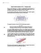
Now the variation of magnetic flux density at different separations of two bar magnets can be found. The two bar magnets should be placed end-to-end to each other with opposite poles facing each other. They are separated by a distance d, as shown on the diagram. The distance can be measured using a metre ruler accurate to 0.5 cm. The distance      

Now the Hall probe can be placed in the centre between the two bar magnets, which are creating a uniform magnetic field between them. The magnets should be placed at a certain, known distance apart. When the Hall probe is placed inbetween the two magnets, the Hall probe will produce a potential difference in the semiconductor wafer which will be shown as a reading. The magnetic flux density of this can be found in two ways; either the magnetic flux density can be read off the graph produced before against the Hall voltage obtained, or the equation derived from the graph can be used:

B = k VH

A table can be made showing the magnetic flux density against the distance at which the result was obtained. At least six values for each should be obtained to ensure that results are reliable. Then a graph can be plotted with the distance (in metres) on the x-axis and magnetic flux density (measured in tesla) on the y-axis. The line of best fit drawn on this graph will show the relationship between magnetic flux density and the distance between two bar magnets.

The magnets should not be mounted using iron clamps, as iron has a high permeability and is magnetic, so would draw flux into it; thereby affecting the results obtained . To cater for the Earth’s magnetic field, the Hall probe can first be used outside of the field of the two bar magnets so that the Earth’s magnetic field can be measured; this result can then be subtracted from each subsequent result obtained to measure the true magnetic flux density of the bar magnets.

---