η = viscosity
c = concentration of spheres
b = constant
exponent γ is greater than 1
The point where these two laws crossover is the point we try to determine in this experiment. At this critical point, all of the polymer molecules are touching and therefore, the size of the individual polymer molecules can be determined. The radius of a polymer molecule can be calculated when concentration, viscosity, volume and relative molecular mass are known, using the equation V = 4 π r³ where V = volume and r =
3
radius for a sphere.
To deduce the conformation of the polymer molecules in solution, we consider the various possibilities of arrangement that the polymer molecules could adopt:
- The molecule stretched out into a straight line. The length of a monomer unit is known to be 0.4 nm and the molecule has about 90 000 monomer units.
- The molecule could be tightly packed into a solid sphere.
-
The molecule could have a loose, irregular coil conformation where successive monomers form a random walk. For this model, the radius of the molecule is known to be: r = a √N where a = monomer length, 0.4 nm and
√6 N = number monomer units, 90 000.
Method:
- 50ml of a solution of PEO and water (concentration 0.625g per 100ml) were placed in a 50ml measuring cylinder.
- Tweezers were used to drop a small black sphere into the cylinder. The time taken for the sphere to fall a known distance was measured, the distance between the 40ml and 35ml marks was used in this first case. Two more spheres were then dropped into the same solution and their falling times for the same distance were measured.
- The spheres at the bottom of the cylinder were then collected using a wire tray. The solution was diluted to three quarters concentration by adding water (new concentration 0.469g per 100ml). Step two was then repeated for each new concentration, for successive new concentrations down to 0.031g per 100ml. Between each different concentration step, the apparatus was washed with warm water.
- As the solution became less viscous, the spheres began to fall more quickly and soon became to fast to time accurately. At each different concentration I tried dropping very small, clear spheres into the solution in the same way as the larger, black spheres. These balls did not fall sufficiently enough to measure until the solution was at a concentration of 0.235g per 100ml. For this concentration, and the next concentration to be tested, I timed both the black and clear spheres. After that point, I timed only the clear. The overlap between the two sets of results gave me a conversion factor between measurements.
Diagram:
Results:
The average time for a 5ml drop for each result was then calculated, as well as the ratio between the two types of sphere.
Ratio of large black spheres to small clear spheres:
1st overlap result = 46.1 = 111.1
0.415
2nd overlap result = 24.9 = 129.7
0.192
Average = 111.1 + 129.7 = 120.4
2
Therefore, multiply values that have only black sphere values, by 120.4 so all values correspond.
Discussion
Einstein’s law states that:
η = η。( 1 + k c )
η = k c η。+ η。
y= mx + c
So for dilute solutions, a plot of viscosity η, against concentration c, should produce a straight line.
We know that viscosity is proportional to time, so a graph of time of falling against concentration should also produce a straight line
We also know that for this experiment that kc>>1, so:
η = k c η。
ln η = ln c + ln kη。
y = mx + c
If a graph is plotted of ln (time) against ln (concentration), we expect a straight line of gradient one.
Gradient of my graph:
Measured from line, gradient = ln 10.9 = 1.04
ln 0.18 – ln 0.08
Error: From results,
Gradient 1 = ln 8.47 – ln 6.53 = 0.641
ln 0.104 – ln 0.069
Gradient 2 = ln 4.16 – ln 2.11 = 1.72
ln 0.046 – ln0.031
Gradient 3 = ln 8.47 – ln 2.11 = 1.15
ln 0.104 – ln 0.031
error = 1.2 = 0.6
2
Therefore, gradient = 1.0 ± 0.6 which is consistent with Einstein’s law.
For larger concentrations, viscosity obeys the law:
η = b c
ln η = γ ln c + ln b
y = mx + c
On my graph, the gradient is therefore equal to γ.
Gradient:
Measured from line, gradient = ln 2500 – ln 20 = 3.41
ln 0.7 – ln 0.17
Error: From results,
Gradient 1 = ln 1810 – ln 773 = 2.96
ln 0.625 – ln 0.469
Gradient 2 = ln 1810 – ln 138 = 4.50
ln 0.625 – ln0.469
Gradient 3 = ln 1810 – ln 46.1 = 1.15
ln 0.625 – ln 0.235
error = 3.4 = 1.7
2
Therefore, gradient = 3.4 ± 1.7 = γ
The graph showed two straight lines, as expected. These two lines joined at the point where the polymer molecules in the solution were all just touching.
At this point, t = 18.5s per 5ml division
Concentration = 0.17g per 100ml error = ± 0.02
Concentration = 1700g per m³ error = ± 200
RMM of PEO = 4×10⁶
1 mole = 4×10⁶g
Concentration = 1700 moles per m³
4×10⁶
Concentration = 4.25×10ˉ⁴ moles per m³ error = ± 0.5×10ˉ⁴
Multiply by avagadro’s number 6.02×10²³,
Concentration = 2.56×10²º molecules per m³
Volume of 1 molecule = __1___ = 3.91×10ˉ²¹ m³
2.56×10²º
For a sphere, V = 4 π r³
3
r = ₃√V¾π
r = 9.77×10ˉ⁸ error = ± 0.60×10ˉ⁸
Therefore, radius of a single polymer molecule = 9.77×10ˉ⁸ ± 0.60×10ˉ⁸ m
Conformations:
-
Molecule stretched out: length = 0.4×10ˉ⁹ × 90 000
= 3.6×10ˉ⁵m
Too big
-
Molecule as tight ball: diameter = monomer length × ₃√90 000
= 1.8 ×10ˉ⁸m
Too small
-
Molecule as loose, irregular coil: r = a √N
√6
= 4.90×10ˉ⁸m
Similar to experimental result.
Therefore, polymer in solution likely to be a loose, irregular coil.
Conclusion
My experiment was successful and I obtained a good result. I verified that viscosity obeys the two laws stated previously. A problem with my experiment was that the qualitative errors stated were too small; the theorized answer lay outside my error margins. A large error in the experiment was with concentration, the solution repeatedly was diluted and any errors increased progressively over time. To make these errors smaller, fresh solution should have been used and diluted each time.
To get a better result, a wider range of different sized spheres could have been used. This would have given more accurate conversion factors. In my experiment, large errors resulted from using the small clear spheres. These spheres were fairly non-uniform in both size and shape and were easily carried by currents resulting from stirring of the solution.
From this experiment, I leant that the size of a polymer molecule in solution is
9.77×10ˉ⁸ ± 0.60×10ˉ⁸ m, and that the shape of this molecule is that of a loose, irregular coil. I also learnt that polymer molecules in solution obey the laws
η = η。( 1 + k c ) and η = b c.