An Empirical Investigation into the Causes and Effects of Liquidity in Emerging

The exchange rate (measured by the nominal exchange rates, adjusted for CPI inflation) measures the trade competitiveness of an economy. This demonstrates the importance of inappropriate exchange rate policies in EMEs, appreciation of the exchange rate will adversely affect the yield spread. This was highlighted in the Latin American capital flight, when sustained real appreciation of the exchange rate of the currencies played a major role in over borrowing. This will reduce liquidity in the long run, as fewer investors will want to hold Latin American debt and the bid-ask spread will widen, because of the increased liquidity premium.

Variables found not to be significant, but may be of interest to consider are changes in international interest rates and oil prices. The 3-month US Treasury bill rate was used to capture the effects of external financial developments. It was hypothesised that this rate would affect the cost of new borrowing and the interest charges on existing debt. Similarly, a supply shock of oil price increases could cause a world recession and increased demand for capital in oil exporting countries (e.g. Russia, Mexico, Indonesia and Venezuela). Hence, it was postulated that a higher real oil price would cause a higher yield spread

Woodward (1983) identified forces that explain the liquidity premium, independent of the shape of the term structure and level of interest rates. The paper also considered whether holding a bond in the short term is more/less risky than holding one in the longer term. The short-term strategy proved to have a lower rate of return, on average, over the near and distant future. Accordingly, implying that the liquidity premium is positive and is affected by individuals’ time-and-state distributed endowments, preferences for risk bearing and consumption, beliefs (and timing of information arrival affecting beliefs) and productive opportunities.

Burnett et al. (1998) examines junk bond (i.e. high-yield) characteristics and behaviour by analysing the influence of economic cycles and periods of reduced liquidity on the behaviour of junk bonds. Of particular interest in this article is the regression of junk and investment grade bond returns against Treasury-bond returns (as a measure of long-term interest rates) and S&P 500 returns (measure of economic activity). This led the authors to the conclusion that large abnormal returns on junk bonds are related to changes in their liquidity. The sensitivity of junk bonds to these variables is also considered, this is because junk bonds are considered to be complex securities that exhibit characteristics of both equity and debt. As follows, their sensitivity changes during the period analysed. During ‘good’ times junk bonds’ returns respond both to Treasury bond returns and stock returns, but are more sensitive to Treasury-bond returns. In ‘bad’ times (economic contraction and high default rates) they are sensitive only to stock returns.

Copeland and Galai (1983) looked at the trade off that market makers must make in deciding how best to optimise their positions. Market makers try to set a bid-ask spread, which will maximise the difference between expected revenues, from liquidity motivated traders and expected losses to information motivated traders. As a result of analysis, it can be proven that the bid-ask spread functions as a measure of market activity, depth and continuity. It also negatively correlates with the degree of competition in the market.

Chordia et al. (2003) looked at stock and Treasury bond markets over a period of more than 1800 trading days. They found that return volatility is an important driver of liquidity and that common factors drive liquidity and volatility in stock and bond markets. For example, through trading activity and asset allocation strategies, shifting wealth between stock and bond markets. A negative ‘information shock’ causes a flight to quality as investors substitute safe assets for risky assets. This could be extremely relevant for policy implications because trading activity in one market could predict trading activity, and in turn liquidity in another. Also leads and lags in volatility and liquidity shocks may have cross – effects. For example, macroeconomic shocks to liquidity and volatility get reflected in one market before another, so that liquidity in one market could influence future liquidity in another. Another interesting relationship they highlight is that unexpected decreases (increases) in the Federal Fund interest rate have an ameliorative (adverse) effect on liquidity as well as volatility.

3. Theoretical framework and variable selection

The theoretical underpinning for this paper is that emerging markets and mature financial markets are more integrated today than at any other time since the First World War.  One indicator of the growing degree of integration is the closer trends of securities prices. The correlation between changes in emerging market bond spreads and changes in US high-yield bond spreads is significantly higher today than a decade ago, despite important differences in the fundamentals underlying the two asset classes. According to Wooldridge et al. (2003), these higher correlations suggest global factors common to mature and emerging markets, rather than local idiosyncratic factors increasingly explain price movements. Thus, it is extremely evident as to why investors are progressively viewing emerging market and US high-yield bonds to be competing asset classes.

Many studies have looked at the returns, yield spreads, volatility and liquidity of bonds in each individual market and what variables affect these measures. However, relatively little work has been conducted into comparing the two asset classes, more specifically comparing the liquidity of them. This paper attempts to compare the two markets to find out if there are cross-liquidity affects and then attempts to seek out which variables affect liquidity of the bonds in each market. This will then enable an analysis as to whether the two markets are inextricably linked via liquidity and whether similar variables affect the liquidity of bonds in each market.

3.1        What is liquidity?

Although many academics will often refer to liquidity in the context of fixed income security markets there is no widely accepted definition of liquidity. O’Hara (1995) as cited in Gwilym et al. (2002) defines it as the ability to trade a security quickly and with little cost. Mackintosh (1995), as also cited in Gwilym et al., suggest that practioners would define a liquid issue as one in which two way markets are available to investors, in reasonable size, over an extended period without undue disruptions or difficulties in establishing fair value. In general Lybek et al. (2002), propose that liquid markets exhibit five main characteristics:

1. Tightness; implies low transaction costs so that pricing information in the market is efficient.
2. Immediacy; considers the time efficiency with which this takes place.
3. Depth; indicates that there are abundant orders from potential buyers and sellers above and below the true price of the security.
4. Breadth; hints that these orders are large and numerous in size.
5. Resiliency; the tendency of markets to correct if prices do not reflect true fundamentals.

3.2        What effects does liquidity have in bond markets?

There has been very little academic research done into role of liquidity in bond markets, but recent crises in financial markets have triggered studies on how to better judge the state of market liquidity and how to better predict and prevent liquidity crises. In particular, the Russian debt moratorium in August 1998 triggered studies by the Bank for International Settlements.

In fixed income markets, a common and systematic source of pricing discrepancy occurs because of illiquid bonds {Gwilym et al. (2002)}. Sarig et al. (1989) as cited in this paper have found further evidence of this. The authors postulate that government bond prices are recorded more accurately than corporate bond prices. This is because of the higher liquidity in the government bond market and higher uniformity of traded assets. Also in this article, Amihud et al. (1986) found that a difference in the liquidity of US Treasury Bills and US Treasury Bonds affects yields to maturity. This leads them to conclude that expected returns are a decreasing function of liquidity because investors require compensation for higher transactions costs in less liquid markets.

Kalimipalli et al. (2002) considered the relationship between liquidity and volatility in the corporate bond market. They found that in general, higher volatility in the returns on assets has two implications for investors: firstly, that they face a higher inventory risk on account of imbalances in their portfolios due to uncertainty in the market and secondly, that they face a higher possibility of dealing with informed traders. As a result bid-ask spreads are wider, so bonds are illiquid. In summation, a positive relationship between volatility and illiquidity exists that could indicate either a higher adverse selection component or a transitory component, or both.

Thus, it is very informative for investors to consider the liquidity effects of the bonds they purchase. More specifically to this paper it is of interest to see how these liquidity effects come about and how, indeed if at all they affect investors choices.

3.3        How to measure liquidity?

Sarr et al. (2002) explain that liquidity measures classify into four main categories:

1. Transaction cost measures that capture costs of trading in the financial assets and any frictions in the secondary markets.
2. Volume-based measures look at the volume of transactions rather than price variability, mainly in order to capture depth and breadth of the market.
3. Equilibrium price-based measures try to capture movements towards equilibrium prices to measure resiliency.
4. Market-impact measures attempt to differentiate between price movements from liquidity of other factors and movements relating to the release of new information in order to measure elements of resiliency and speed of price discovery.

There is no single measure that unequivocally measures tightness, immediacy, depth, breadth and resiliency.

The bid-ask spread is a measure that is frequently used in econometric analysis of fixed income markets. It is a transaction cost technique of measuring liquidity using the difference between the price of buying and selling the asset in question. This measure captures order-processing costs, asymmetric information costs, inventory-carrying costs and oligopolistic market structure costs. Owing to the fact that all of these types of cost are encapsulated in the bid-ask spread, the measure also takes into consideration some factors of immediacy, breadth and resilience. This is mainly because, if the costs described above are low, then there will be a high number of market participants.

The bid-ask spread can be expressed as the absolute difference between bid and ask prices or as a percentage spread (equations 1 and 2 respectively below). A narrow spread suggests a greater liquidity because the market price of the bond is more accurately reflected and thus easier to sell in the market. The percentage spread takes into account the fact that a given spread would be less costly the higher the prices and it is easier to compare across markets:

1. S = (PA – PB) where PA is the ask price and PB the bid price
2. S = (PA – PB) / ((PA + PB)/2))

Volume-based measures have also been used in many studies of liquidity, however, they do not provide the variety of information in their values as is incorporated in the bid-ask spread. For example, such measures do not include the cost of trading, which is taken into account by the bid-ask spread. Volume measures can also give distorted results; for example when liquidity is low, volume could be high if transactions costs are high. This has been discovered to occur particularly around earnings announcements. Several authors quoted in the Alexander et al. (2000) article comment on the ‘speculative’ component of volume and explain it as difference in opinion on the true value of the financial asset.

Thus, in this analysis the bid-ask spread as represented by equation (1) is used. Although, this does not contain as much detailed information as the percentage spread {equation (2)}, owing to the availability of data so this measure of liquidity is applied.

3.4        What affects liquidity?

In the light of previous literature and studies that have focused on liquidity, and EME and US corporate debt, the following variables are considered in this analysis:

The interest rate available on US securities is clearly of fundamental importance to both types of debt. However, as observed in earlier studies, different Treasury securities have different effects on bond spreads and capital flows, and thus will probably have different effects on debt liquidity.  Kamin and Kleist (1999) suggest that lower interest rates in the US make risk on EME debt look more attractive and increase investor risk tolerance. The empirical findings of Ferrucci et al (2004) confirm this, with US 30-day Treasury Bill yields’ having a large significant positive effect on EME bond spreads. Min (1998) used the 3-month US Treasury Bill Rate to capture the effects of external financial developments and its effect on capital flows to developing countries.  Min found this proxy of world interest rates to be insignificant in influencing capital flows to developing countries in the 1990s. Finally, Ferrucci et al (2004) also find that higher long-term (10 year) US interest rates have a strong negative impact on EME bond yield spreads. This result suggests that the effect of a steeper yield curve on leveraged investors’ incentives was greater than the long-term cost of borrowing to EMEs. Thus, it is for this reason the yield on 10-year US government bonds is used as a measure to capture the cost of investing in EME sovereign and US high-yield corporate bonds and the affects on their respective liquidities.

Inflation was also found to have a significant impact on debt, particularly EME debt, thus, it will be interesting to see if it also affects US corporate debt liquidity. Higher inflation erodes the return of bonds. Both EME and US high-yield bonds are dollar denominated, therefore the US Consumer Price Index (CPI) is used as a variable in order to consider inflationary consequences.

Other variables that are interesting to consider are the US S&P 500 equity index and NASDAQ Composite Index. They provide key measures of economic activity and the opportunity cost of lending because investors could instead be holding shares. Correspondingly, these measures will potentially have a large effect on the liquidity of the two types of debt. The NASDAQ Composite Index represents all stocks that trade on the NASDAQ stock market. Most are technology and internet related, but there are financial, consumer, biotechnology and industrial companies as well. For that reason, the companies listed show high growth potential, but because of this are more speculative and risky than those on the NYSE. This makes the index more volatile than other broad indices, such as the S&P 500. This index is considered to be the benchmark of the US stock market. It attempts to cover all major areas of the US economy. Not necessarily the 500 largest companies, but rather the 500 most widely held companies, chosen with respect to market size, liquidity and industrial sector.

Another variable that could cause liquidity effects is the world oil price (West Texas Intermediate Spot Oil Price as a measure for this). There are many different varieties and grades of crude oil, buyers and sellers, therefore find it easier to refer to benchmark oils. In the United States, the benchmark is West Texas Intermediate (WTI), thus sales into the US are usually priced in relation to WTI. Therefore, the WTI benchmark will be most significant to this analysis. Many EMEs remain dependent on a few primary commodities for a large part of their export receipts, and the single significant commodity is oil, accounting for around a third of commodity exports from the major EMEs. The largest exporters of the commodity are Venezuela, Russia, Mexico and Indonesia. Similarly, many EMEs are big oil importers, such as China, Brazil and Korea. This means that any changes in oil price could also have significant consequences on their fiscal positions, potentially leading to changes in their external debt liquidity. Many of the U.S corporates that issue high-yield bonds are also based in the energy sector, which is one of the top five industry groups that issue high-yield debt. Even if the high-yield corporates are not in the energy sector, they may suffer the consequences of changes in oil prices.

One other variable that could affect the liquidity of both types of debt is some measure of volatility of equity. The Chicago Board of Exchange publishes an index (VIX index) that measures market expectations of near-term volatility conveyed by S&P 500 stock index option prices. Since its introduction in 1993, VIX is considered by many to be the world’s premier barometer of investor sentiment and market volatility. This variable has not been widely used before in studies conducted on fixed income markets, but may be of some interest.

Finally, the cross-liquidity effects of each type of debt are examined, by noting how the bid-ask spreads on one type of debt affect the bid-ask spreads on the opposing asset class. The intuition behind this is that if EME debt is liquid then investors will convert to holding this type of debt and vice versa with US corporate debt.

4. Description and analysis of data

There are two issues related to the construction of data for this empirical investigation: the selection of appropriate sources for the bid-ask spreads on emerging market and US corporate debt and the choice of a set of explanatory variables.

4.1        Choice of data

In this paper, in order to compare the two asset classes which form the basis for the dependent variables, indices of the sovereign bonds in emerging economies and corporate bonds in US high-yield markets are analysed. The index used for emerging market sovereign bonds is the JP Morgan Emerging Market Global Bond Index (EMBI-G), which is a widely used benchmark for investors and allows a broad representation of the types of instruments available in emerging bond markets. The index reflects the fact that the indices are intended principally for portfolio management purposes, country spreads being weighted together according to the size of their underlying debt market.

The EMBI Global is a relatively new index to be released by JP Morgan, following on from their EMBI and EMBI+ indices, covering a yet-wider range of emerging economy instruments. As stated in Cunningham (1999), the definition of an emerging economy is broader: ‘All countries classed as low or middle income by the World Bank and any others who have restructured debts over the last ten years.’ i.e. there is no set level of credit rating the debt has to have.

The index only covers instruments with a face value of over US$500 million and at least two and a half years to maturity, mainly Eurobonds and Brady bonds. Bonds must also pass a liquidity test, that is, there must be a daily price available from either JP Morgan or another source. This is vital to this analysis because some emerging country bond markets are not so liquid; therefore quoted prices do not reflect actual trades.

Thus, the countries included in this index are as follows: Argentina, Brazil, Chile, Colombia, Ecuador, Mexico, Panama, Peru, Venezuela, China, Indonesia, Malaysia, Philippines, South Korea, Thailand, Bulgaria, Croatia, Hungary, Poland, Russia, Algeria, Egypt, Greece, Ivory Coast, Lebanon, Morocco, Nigeria, South Africa and Turkey. In total 183 individual bonds issued by these countries are included in the index. This allows wider world coverage than previous indices constructed by JP Morgan, which traditionally had a heavy Latin American weighting. The most heavily weighted bonds in the index are Russian, Brazilian, Venezuelan and Mexican sovereign issues.

In order to provide a suitable comparison of emerging debt with US high-yield corporate debt, the Merrill Lynch US High Yield Fund Index is used. This offers a very similar set of criteria to EMBI-G for bonds to be included in the index, allowing an exact comparison to be performed. According to the Merrill Lynch website, the primary objective of this fund is to obtain current income. As a secondary objective, the fund seeks capital appreciation, when consistent with its primary objective.

The criteria for inclusion in this index is for fixed income securities that are rated Baa, or lower, by Moody’s Investors Services, or BBB, or lower, by Standard & Poor’s. That is, all bonds must have a credit rating below investment grade but not in default. Although the JP Morgan EMBI Global does not have a set ‘rating criteria’ for inclusion, the debt in both indices is of a similar rating. A large proportion of the EMBI Global index debt would not have a rating of Baa/BBB or above. The five industries most heavily weighted in the Merrill Lynch index are: chemicals, utilities, energy (other), food & tobacco and gaming. Bonds will typically have at least one year remaining until maturity.

For the choice dependent variables monthly averages of daily closing prices for each variable, from 1/1/1998 to 31/8/2004, are used, giving a sample size of 80. The reason daily data was not used is because of its volatility and noise in almost all of the time series. By averaging the data on a monthly basis the noise was greatly reduced, still allowing an adequate sample size. The timeline chosen is to incorporate the start publication of the EMBI-G index by JP Morgan, at the beginning of 1998, which takes into account recent currency crises that are of interest in monitoring the reaction of investors during liquidity changes occurring throughout these crises.

Data for the whole of the Merrill Lynch High Yield Fund Index proved to be too large, as there are thousands of bonds listed in the index. Thus, in order to obtain a representative sample that was easily workable, the top 200 bonds by market capitalisation are used. This is similar to the number of bonds in the EMBI-G index so that their averages are comparable. Another problem encountered, was that during the 6 year period, bonds frequently drop in and out of the Merrill Lynch index. In order to allow for this, a snapshot of the bonds that were included in the index from the 31st January 1998 was taken and these are the bonds that monthly averages are given for up to 2004. This is to ensure that the bonds have a life span of at least the 6-year time period considered.

The explanatory variables of the model include the yield on 10 year US Treasury securities, the US S&P 500 equity index and NASDAQ Composite Index, the CPI in the US (as a measure of inflation), the VIX index (that measures market expectations of near-term volatility conveyed by S&P 500 stock index option prices) and the West Texas Intermediate Spot Oil Price (as a proxy for world oil price).

4.2        Analysis of liquidity data

It is interesting to consider, in the first instance, the changes in liquidity in each of the bond indices, based on the impact of global macroeconomic events before performing any further econometric analysis.

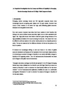
Emerging Market Sovereign Bond Liquidity

As is evident from figure 4.1 there was a large period of illiquidity spanning from August 1998 to September 2000 in emerging market sovereign bonds. This marked a

period just after the Asian crisis had ensued, mid-1997 whilst continuing to impair growth throughout 1998. In the summer of 1998 there was also economic and political crisis in Russia. This coupled with the devaluation of the Brazilian real in Jan 1999 marked a period of 3 years of solvency and liquidity problems in emerging economies. There was a large reversal of private capital flows to emerging economies and increased evidence of capital flight from investors, with their focus being that of retreating from risk. This led to a reduction in total exposure of investors to emerging markets and in particular reduced leverage, thus triggering this illiquidity in emerging sovereign bonds.

Figure 4.1

In 2002 emerging bond markets rallied, outperforming most asset classes and huge inflows were made into the secondary bond markets. Inflows had been postponed prior to this in anticipation of the Argentine crisis, but there was a lack of contagion because investor concerns had been building for some time. Thus, dedicated investors had taken underweight positions in risky credits (e.g. Brazil) and overweight positions on relatively immune credits. A new, reasonably large issuance was made by emerging markets in May 2002, following an 11 week drought from the Russian crisis. Ensuing were the, afore mentioned, huge inflows of investors, with increased allocations from crossover investors, although with still comparatively underweight positions in Argentina. This led to, a development in investor’s understanding of dollar denominated emerging sovereign bonds and a significant improvement in liquidity.

This improved awareness continued through into 2003/2004 where there was a greater stability in liquidity of these bonds. Indeed, emerging bonds posted impressive returns in 2003. A highly accommodative monetary stance in the main industrialised countries contributed to a search for yield amongst investors that continued to encourage sizeable inflows into the secondary emerging bond markets. The start of 2004 saw strengthening fundamentals in emerging economies, with surging commodity prices, fiscal consolidation in key countries, increased foreign reserve holdings and shifts to floating exchange rates. This was reflected in a number of credit rating upgrades in significant members of the EMBI-G: Indonesia, Russia, South Africa and Turkey. This contributed to sustained liquidity in the market.

US High-Yield Corporate Liquidity

Figure 4.2

During 1998, conditions in credit and liquidity of markets in the US were extremely poor. This was mainly because of the Russian and Long-Term Capital Market crises in autumn 1998, which raised the cost for US corporations of raising finance through bond markets. Although perhaps there was no rise in perceived risk on US corporations, bond investors increased their levels of risk aversion. Similarly, during periods of market turbulence bond investors attach more importance to liquidity, bidding up the price of government bonds relative to less liquid corporate bonds. Hence the extremely wide bid-ask spreads at the start of 1998.

However, 1999 saw market conditions improve. In particular, bond market implied probabilities derived from options prices edged down after sharp increases in the latter half of 1998. Market risk was also substantially reduced in 1999, demonstrated by the reopening in the market for high-yield debt with several companies even being able to tap into international markets in Euro and Sterling denominated debt.

The period from September 2000 until February 2001 then saw a sustained phase of illiquidity. This was due to a number of key factors. Firstly, there was a large increase in the default rates of high-yield corporate debt. This could have been owing to the fact that corporate profits started to fall at the end of 1999 and continued to do so into Q1 2001. A second cause could have been the huge issuance of high-yield bonds in 1998, originally helping to increase liquidity in the market. However, default rates peak on such bonds 2-3 years after issue and given the lower issuance since that time, credit quality and hence liquidity in the market began to fall.

Other reasons for this period of illiquidity could have included the changing structure of US industry at this time, with a growing importance of investment in information and communications technology. This also resulted in increased default rates, particularly in ‘sunset’ industries and young start-up enterprises in novel sectors, which would be most likely financed using high-yielding debt. Thus, the increased volatility in the market during this period meant that the interest rates on new bond finance for speculative grade issuers was greatly increased, mainly due to the tightening of credit standards.

From the start of 2002, changing perceptions of the economic slowdown and prospects for recovery dominated global market developments. It was felt that financial markets had overreacted to the potential impacts of the September 11th attacks in 2001. Subsequently, there was a rally on all financial markets with ample liquidity provided by investors.

With the risk appetite of investors being at its highest level in two years and oil prices remaining low, a sharp sell-off in the US bond markets occurred. This caused a narrowing of bid-ask spreads in the high-yield markets, which matched a similar pattern on emerging market bonds.

This ample liquidity continued to dominate mature financial markets into 2003/2004, where it is evident from Figure 4.2 that liquidity in the US high-yield bond market stabilised. Mature market vulnerabilities had eased significantly with investors increasingly prepared to assume credit risk and interest rate risk in the search for yield. This led to high investor inflows into US corporate bonds, with signs of reduced investor discrimination between low and high rated issuers. Measures taken by corporations to cut costs, defer investment and strengthen balance sheets helped to amplify this, as well as the resurgent economic growth and higher corporate earnings.

5. Empirical analysis and results

5.1        Unit Root Tests

All of the time series data were tested for unit roots using the Augmented Dickey Fuller (ADF) test, employing the general-to-specific approach in order to identify the correct ADF specification to use. 

        ∆yt = δ + ρyt-1 + ∑ βi ∆yt-i + Ut

H0: ρ = 0 {I(1)} – Non-stationary time series

H1: ρ < 0 {I(0)} – Stationary time series

Only one time series displayed stationarity, namely the Chicago Board of Exchange Volatility Index. Consequently, this variable is not used in any of the cointegration analysis because it is I(0) and therefore cannot generate cointegration and is assumed to be exogenous to the model. Perhaps this is why no previous studies have considered this variable in examining emerging market bonds and US high-yield corporate bonds. All other variables contain a unit root and are non-stationary, that is, do not revert to a mean value. For this reason, it is possible that cointegration between any of the other variables could exist.

5.2        Hypothesis 1: Do cross-liquidity effects exist between the two markets?

First, the hypothesis that the EMBI-G and Merrill Lynch bond indices have cross-liquidity effects was tested. In order to do this a single equation cointegration approach was used (as described by Engle and Granger (1987)).

The following result was obtained:

Equation 5.1

yt = 0.326959 + 0.330581 x1 + εt

         (0.02563)           (0.06831)

The standard errors are shown in brackets

Where

yt = Bid-ask spread on EMBI-G

α = A constant

x1t = Bid-ask spread on Merrill Lynch US high-yield fund

εt = Residuals

The residuals of this equation do not contain a unit root, implying that cointegration exists between the liquidity of the two markets. In terms of economic interpretation, this means that there is a long-run relationship between the two variables that is worth investigating. Once cointegration has been found to exist, standard OLS procedures can be conducted. The β estimate is statistically significant at the 1% level and suggests that as liquidity in the EMBI Global Index increases by 1%, the liquidity of the Merrill Lynch Index increases by 0.330581%. This also holds theoretically because of the fact that the two bond markets are competing asset classes. Thus, a sell-off in one market will probably be as a result of investors switching their positions into the opposing market.

This can be examined graphically:

Figure 5.1

As is evident from this figure, the liquidity on the two types of bonds do follow similar cycles, although a time lag appears to exist in the US high-yield spread that is gradually evened out into 2003.

This is even more apparent if the residuals of the regression are analysed graphically:

 Figure 5.2

From Figure 5.2 it is apparent that when the residuals of the Equation 5.1 are negative, the EMBI Global bonds were more liquid than the US high-yield bonds. As the bonds became more illiquid, liquidity in the US high-yield index improved considerably. This implies that over time (in the long-run) liquidity of the two bond indices will offset one another so that they will always revert back to a mean overall level of liquidity. The two types of securities are inextricably linked via their cross-liquidity effects.

5.3        Hypothesis 2: Do similar variables affect liquidity in both markets?

This single equation approach does however have limitations in that it is not the most efficient estimator of the relationship between the variables. Therefore, in order to better estimate the relationship and incorporate a number of explanatory variables, the single equation approach is extended to a multivariate framework. The Johansen technique (Johansen 1988) is used in order to do this. Firstly a vector is designed, allowing all of the variables to be potentially endogenous:

zt’ = [ y1t, y2t, y3t, y4t, y5t, y6t, y7t]

where

y1t = Bid-ask spread on EMBI-G

y2t = Bid-ask spread on Merrill Lynch US High-Yield Fund

y3t = Yield on 10-year US Treasury Security

y4t = S&P 500 equity index

y5t = CPI in the US

y6t = West Texas Intermediate Spot Oil Price

y7t = NASDAQ equity index

The VAR is first estimated as an unrestricted system using the Ordinary Least Squares method (OLS). The model is correctly specified with 4 lags, so that the VAR framework is given by:

zt = A1zt-1 + A2zt-2 + A3zt-3 + A4zt-4 + Ut   where Ut ~ IN (0, ∑)

Measures of goodness of fit of the unrestricted system suggest that the model has a good specification relative to the data. F-Tests on the model also suggest that unrestricted regressors were statistically significant and that the retained regressors with a lag length equal to 1 were statistically significant at the 1% level. Thus, all regressors are important to the construction of the model.

The model is then tested to determine how many cointegration vectors exist, in order to do this the Johansen reduced rank regression approach is used (Johansen 1988) and the trace test is applied. This involves a sequential testing procedure, so that:

Trace Tests for the Unrestricted VAR

NB: *  significant at 5% level

        **significant at 1% level

Table 5.1        

This shows that there are 3 cointegration relationships in the model. Thus the VAR can be re-specified as a cointegrated VAR of rank 3, including the cointegration relations, so that designed zt converges with its long-run steady state solutions. This implies that there are 3 disequilibria in the model.

The VAR(3) can then be reformulated into a Vector Error Correction Model (VECM) form:

∆zt = Γ1∆zt-1 + Γ2∆zt-2 + Γ3∆zt-3 + Πzt-1 + Ut

where

Γi = - (I – A1 – A2 – A3), (i = 1, 2, 3)

Π = - (I – A1 – A2 – A3 – A4)

The Π matrix contains the most useful information on short- and long-run adjustment to changes in zt and can be broken down into two parts so that Π = αβ where β contains information on long-run adjustments to disequilibrium and α contains information on the speed of adjustment to equilibrium.

By examining the normalised β values contained within the Π matrix, equations can be formed that describe the model in the long-run when it is in equilibrium. Due to the fact that there are three cointegration vectors, three equilibria exist for the VECM:

Equation 5.2 – First Equilibrium

y1t = 0.14665y2t – 0.13360 y3t + 0.00029598 y4t – 0.0064190 y5t – 0.0029079 y6t + 0.026953809 y7t

where

y1t = Bid-ask spread on EMBI-G

y2t = Bid-ask spread on Merrill Lynch US High-Yield Fund

y3t = Yield on 10-year US Treasury Security

y4t = S&P 500 equity index

y5t = CPI in the US

y6t = West Texas Intermediate Spot Oil Price

y7t = NASDAQ equity index

This equilibrium shows that as emerging market bonds become more illiquid (that is, as the bid-ask spread increases), so also, do US corporate bonds. At the same time the yield on US Treasury securities is falling. So that, a 1% increase in illiquidity of emerging market bonds is associated with a 0.14665% increase in illiquidity of US high-yield corporate bonds and a decrease in yield of 0.13360% on US Treasury securities, in order to achieve equilibrium. All of the other variables show very small amounts of adjustment to changes in emerging market liquidity, which can be considered negligible.

Overall, this equilibrium suggests that as emerging market bonds show illiquidity, (probably as a result of investors holding their positions), US corporate bonds also show signs of illiquidity, which is predominantly caused by a decreasing yield on US Treasury securities. This leads to the conclusion that bonds in both markets will respond to decreasing yield of government securities, (a proxy for lower global interest rates), in similar ways. This is shown by bonds in each market becoming illiquid as investors hold their positions.

Equation 5.3 – Second Equilibrium

y2t = -4.3556 y1t + 0.44641 y3t + 0.00012487 y4t – 0.060029 y5t + 0.051765 y6t – 0.00053265 y7t

This equilibrium produces slightly different results to the first, it is evident that a 1% decrease in liquidity of US corporate bonds, (a bid-ask spread increase), will be associated with a 4% increase in the liquidity of emerging market bonds and an increase in yield on US Treasury securities of 0.44641%. This is contrary to the results from the previous equilibrium, perhaps because this equilibrium is achieved by an increase in yield of US Treasury securities, rather than a decrease as before.

This equilibrium also shows larger coefficients on other explanatory variables. A 1% decrease in liquidity, is accompanied by a 0.06% decrease in the US consumer price index and a 0.05% increase in oil price. These coefficients suggest improved macroeconomic conditions for firms in the US, particularly those in the energy sectors, which is the sector some of the most heavily weighted corporates in the Merrill Lynch High-Yield Fund Index are part of.

Thus, it is possible to argue that a yield increase on US Treasury securities encourages investors to hold their positions on US high-yield corporate bonds, especially accompanied by a decrease in the US CPI and oil prices. However, the

yield increase on US Treasury securities/global interest rates, causes increased liquidity in emerging market bonds, probably as a result of a sell-off in this market, as conditions in the opposing asset class improve.

Equation 5.4 – Third Equilibrium

y3t = -20.709 y1t – 22.869 y2t + 0.011512 y4t – 0.11023 y5t – 0.081368 y6t – 0.00040677 y7t

This equilibrium provides different results again. The variables that show the greatest response to a 1% increase in yield on US Treasury securities are emerging market and US corporate bond liquidities. This time the magnitude of the changes is much larger, with a 20.709% increase in liquidity of emerging market bonds and a 22.869% increase in liquidity of US corporate bonds. Emerging market bond liquidity has the same response to an increase in yield on US Treasury securities, as predicted by the second and first equilibrium. However, US corporate liquidity does not respond to increasing yield on US Treasury securities as it does in the second equilibrium.

The reason for the surprising results may be the increased coefficients on the other explanatory variables. The third equilibrium sees an increase of the S&P 500 index level by 0.01%, a decrease in US consumer prices of 0.11% and a decrease of oil price of 0.08% related to a 1% increase in the yield of US Treasury securities. This perhaps makes both US corporates and emerging market bonds seem less attractive to investors, thus liquidity on both bonds increases significantly as a sell-off in each market occurs.

The speed of adjustment to the three equilibria in the model can also be examined. This is given by the estimated values of α:

Speed of Adjustment Matrix Results

NB: *  significant at 5% level

        **        significant at 1% level                                    

   

Table 5.2 

The estimated α values suggest that out of the explanatory variables, S&P 500 equity index is the quickest, most significant variable in responding to the second and third disequilibria in the model, in order to generate cointegration. The yield on a US 10-year bond is also significant in adjusting to all three of the disequilibria, but is substantially slower than the S&P 500 index in doing so. It is also apparent that the liquidity measures of the two bond indices show very slow response times to disequilibria. With significance attached to the response of the EMBI-G liquidity to changes in the second disequilibrium at the 1% level and the response of US corporate liquidity to the first disequilibrium at the 5% level.

Overall, this perhaps suggests that investors are quite slow to react to changes in liquidity in the bond markets, but the changes are significant when disequilibrium involves the opposing asset class. Similarly the yield on US government securities has a slow but significant impact on deviations from all of the equilibria, that is, the equilibria involving both types of bond security. However, the S&P 500 equities will respond quickly to changes in the second and third equilibria of the model, that is, those including US corporate liquidity and the yield of the US government securities.

To provide further analysis of the model tests for weak exogeneity and linear restrictions on the cointegration vectors were undertaken. It was found that the likelihood ratio test of restrictions that US CPI, Oil Price and NASDAQ are weakly exogenous to the model, (that their α coefficients = 0), could not be rejected. This in effect means that these variables do not adjust to any of the disequilibria in the short run and only have long run effects on the model.

In order to clarify the effects of the other variables that are endogenous, the model was re-estimated using the vector zt given as:

zt’ = [ y1t, y2t, y3t, y4t]

where

y1t = Bid-ask spread on EMBI-G

y2t = Bid-ask spread on Merrill Lynch US High-Yield Fund

y3t = Yield on 10-year US Treasury Security

y4t = S&P 500 equity index

        This model is correctly specified with 3 lags and the trace test confirms that two cointegration vectors exist in this model. Restrictions were then placed on the normalised β matrix in the model, in order to identify a unique cointegration vector that fully describes the impact of the variables in zt. The results obtained from this analysis were as follows:

Identified β Values (adjustment to disequilibrium):

       Table 5.3

NB: *  significant at 5% level

                                                                        ** significant at 1% level

                                                        

Identified α Values (speed of adjustment):

         Table 5.4

This analysis can lead us to further, more conclusive analysis of the variables that affect liquidity on both markets.

It is evident from the identification of the unique cointegration vector, that the only variable that has both a short and long term effect on the liquidity of emerging market bonds is the liquidity of US corporate bonds. This can be represented by the first column of the identified β matrix and the equation:

Equation 5.5

EMBI-G liquidity = - 0.6208 US Corporate liquidity

So that as US corporate bonds become more liquid, the liquidity on emerging market bonds will decrease. This is a conclusion that has been fundamental to the paper and was examined under hypothesis 1, thus is fully empirically supported.

The second part of the identified cointegration vector provides the most interesting analysis. This can be represented by the second column of the identified β matrix and the equation:

Equation 5.6

US Corporate liquidity = -0.072202 yield on US Treasuries + 0.01374121 S&P 500

This shows that US corporate bond liquidity is affected exclusively by the yield on 10-year US Treasury bonds and the S&P 500 equity index in the short and long run. This implies that in the short term it is in fact US corporate bond liquidity that affects emerging market bond liquidity and not vice versa. US corporate bond liquidity is affected mainly by the yield on Treasury securities and the S&P 500 equity index.

5.4        Empirical Conclusions

Overall, by using econometric techniques to show where cointegration exists between the variables, the theoretical foundations of this paper can be empirically supported. Evidence is provided throughout the data time series to support hypothesis 1 that cross-liquidity effects do exist between the two bond markets. Further analysis towards the end of this chapter describes that in the short run it is US corporate bond liquidity that moves first, affecting emerging market bond liquidity to bring the two markets back into equilibrium.  US corporate bond liquidity is affected by changes in macroeconomic conditions in the US. In both the short and long run this is mainly concentrated in changes of yield on 10-year US Treasury securities, which is a proxy for global interest rates, and the S&P 500 equity index, which is a measure of economic activity. Evidence shows that emerging market bond liquidity is also affected by the same two variables, although perhaps only in the long run, and probably through the effects the variables have on the liquidity of US corporate bonds.  The other explanatory variables of the model also contribute to liquidity changes on the two bond markets, however, they are found to be weakly exogenous to the model. This suggests that their importance is limited to their long run effects on the yield of 10-yr US Treasury bonds and the S&P 500 index, which in turn effect the liquidity of the bond markets under consideration. As a consequence, it is possible to say that hypothesis 2 is also empirically supported and similar variables do affect the liquidity of both bond markets. Although, this may be provided by the cross-liquidity effects each type of bond has on the opposing asset class.

---

6. Conclusions and Policy Implications

Several developments in financial markets over the past decade have provided the impetus for the empirical investigation of this paper. Firstly, the growth of issuance in emerging market sovereign bonds by many developing countries has triggered much interest surrounding the volatility of investing in such debt. Particularly relevant to the context of this paper is the liquidity constraints of holding such debt and how this effects investors choices. Similarly, it is important to consider the potential financial stability implications of the governments in developing economies relying heavily on bond issuance as a form of financing government spending.

Secondly, the past decade has seen emerging sovereign bonds and US high-yield corporate bonds become increasingly competitive asset classes, mostly as investors have been engaged in a search for higher returns and yields in their portfolios following low global interest rates.

In the light of these developments this paper examines two main hypotheses:

• Are emerging market sovereign bonds and US high-yield corporate bonds linked via their cross-liquidity effects.
• Do similar variables affect the liquidity on each type of bond?

 In order to investigate these hypotheses bid-ask spreads for the period January 1998 – August 2004 on JP Morgan’s Global Emerging Market Bond Index and Merrill Lynch’s High-Yield Fund Index were examined and placed in a multivariate cointegration framework with the explanatory variables of yield on 10-year US Treasury securities, US CPI, S&P 500, Oil Prices and NASDAQ. Another variable of Chicago Board of Exchange Volatility Index was found not to contain a unit root, thus would not generate cointegration in the model and was assumed to be exogenous.

The first hypothesis, that emerging market bonds and US high-yield corporate bonds are inextricably linked via their cross-liquidity effects was proven using the single equation Engle-Granger cointegration technique and the Johansen multivariate technique. From the identification of a unique cointegration vector, using the Johansen technique, it is accurate to say that a 1% decrease of liquidity on emerging market bonds will cause a 0.68208 increase in liquidity on US high-yield corporate bonds.

Three variables are found to be weakly exogenous to the model: US CPI, Oil Prices and NASDAQ. This identifies that they do not have an affect on liquidity in the short run, but affect liquidity in the longer term through their influence on other variables. For this reason a new model was constructed, only placing the liquidity of each bond, yield on 10-year US Treasury securities and S&P 500 in a multivariate framework. This allowed the identification of a unique cointegration vector, permitting firm conclusions. The conclusions reached are that both yield on US Treasury securities and S&P 500 have an impact on US corporate liquidity and through the cross-liquidity mechanism have an effect on emerging market bond liquidity. Thus, the second hypothesis that similar variables affect the liquidity of each type of bond is proven, although perhaps in a more indirect fashion.

6.1        Policy Implications

The policy implications of this analysis are quite varied and far-reaching. Bond market liquidity is very important for emerging markets because it affects the operation of monetary policy and contributes to financial stability. According to the APEC website if market liquidity is not sufficient, central banks might not be able to provide or absorb the necessary amount of funds smoothly through their open market operations. This could produce unintended effects such as excessive price volatility.

In a wider context bond market liquidity facilitates instruments of financial intermediation, which encourages efficient market pricing, as well as economically efficient borrowing and investment decisions. This is vital for both emerging markets and US corporations, if a liquid market for raising cost effective debt financing does exist then sovereigns and firms are provided with valuable financial flexibility.

However, there is a serious downside if a country or firm faces unsustainable debt. Private creditors have become increasingly numerous, anonymous and difficult to coordinate. The problem is exacerbated by the variety of debt instruments now available in both markets, and in the case of emerging market bonds the range of legal jurisdictions in which debt is issued.

The IMF, in its debt restructuring fact sheet, outlines how countries facing severe liquidity problems will go to extraordinary lengths to avoid restructuring their debts to foreign and domestic creditors, because they realise that even an orderly debt restructuring can sever access to provide capital for years, leading to crisis. As a result, countries with unsustainable problems will wait too long before confronting them, which is harmful to the country, its citizens and the entire international community. The cost of default is driven even higher because the current international financial system lacks a strong legal framework for the predictable and orderly restructuring of sovereign debt.

Bearing this in mind short-term investors in both markets should be willing to pay premiums for liquid bonds and if they choose to hold positions on illiquid bonds they should closely monitor global interest rates and economic activity for potential liquidity problems. Similarly, it is important to monitor the political climate surrounding the purchase of both types of asset because analysis in chapter 4 shows liquidity problems around times of crises.

Longer-term investors should be prepared to accept losses because of the problems of liquidity in certain economic climates and around times of crises. This is particularly pertinent if there is significant chance of default on the bonds. For such investors; US CPI, Oil Prices and NASDAQ may be additional valuable tools in monitoring potential liquidity changes.

Turning to emerging market governments and US corporations that use these bonds as ways of raising finance, it is evident that investors are increasingly turning to such assets in the construction of their portfolios, because of the promise of greater returns. However, such issuers need to be careful because very small changes in the economic climate, that are not under their control, can cause changes in liquidity that could cause sell-offs of their assets. If there is also a lack of confidence in a particular emerging market, or US corporate, that is relying on these bonds as a source of finance and a sell-off occurs, it is difficult to find alternative sources of finance and a large risk of default could be imminent.

With an increase in the purchase of these types if bonds it has also become more important for the individual countries to monitor exactly how much domestic firms are investing in such issues. Particularly if the risk of default on these types of bond is high, financial stability risk for institutions that purchase the bonds could affect financial stability for the whole country, especially if unexpected crises occur.

6.2        Further Research

The extensive conclusions of this paper lead to the possibility of more research on this topic. It would be interesting if further proof could be examined on exactly how investors react to changes in the variables considered in this paper. This is possible by looking at levels of issuance and purchases of both types of bond and comparing them to the explanatory variables, and then liquidity of the bonds. This would add further conclusive evidence to what causes periods of liquidity and illiquidity.

A sensitivity analysis of the liquidity on such bonds may also provide some insightful interpretations as to whether liquidity is more sensitive to changes in stock markets, or interest rates. In addition, the sensitivity of liquidity to periods of market stress and the reaction of individual bond issues to such periods, particularly bonds with the highest market capitalisations. Another point of curiosity would be to examine the relationship between liquidity and volatility of such categories of bonds and an interpretation of how the two are related.

To conclude, as emerging markets become more closely integrated with the developed world through financial markets and begin to compete with incumbent players, such as US high-yield bonds, it is important that the relevant precautions are taken to ensure that financial stability is prevalent. In the case of secondary bond markets, this is especially important, because of the implications for investors purchasing such issues and the entities issuing them.

---