Restaurants and fast-food chains will often want to express their break-even point by the number of portions sold. This is fairly easy to compute. Here, the break-even point is determined by applying the following formula: break-even point (in units) equals Total Fixed Cost divided by (selling price per unit minus variable cost per unit).
If the selling price of a steak is $1.20, the total fixed cost is $30,000, and the variable cost per unit is 80 cents, how many units must be sold to break-even?
If we apply the formula, the break-even point is
Using this formula, we can compare different sale prices. The break-even point for each price will be calculated and an analysis of the results will determine how reasonable they are and which is to be used when forecasting and budgeting.
Another possibility that the break-even point offers is for a study of the relation between the revenue and cost. A chart can be drawn showing the total revenue and cost at different levels of production when selling a hamburger or a drink at a specified price.
The break-even point graph helps the business owner determine the levels of production that will create profits for every level of sales. The business owner then works to increase profits without investing extra funds. To do this, he/she should study the following important points:
- A possible increase in utilization of existing capacity through reduction of idle time.
- Better repair and maintenance of equipment to reduce down time --time elapsed from the moment the machine breaks down to the time it gets back in service.
- Improved working schedules and inventory levels.
- Longer business hours.
- Improved production control.
- Mark-up policy.
(M2)Evaluate planning and control methods used in engineering project
-
Planning Methods; What’s planning? It’s the sum of setting the goals of an engineering company, forecasting the environment in which the engineering company will operate and determining the means to achieve the goals. Once the goals have been refined and change in the light of environmental casting then plans can be made to achieve the goals. For this reason, plan can be categorized into different methods.
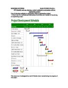
-Schedules; Project planning is different from other forms of planning and scheduling because the set of activities that constitute a project are unique and occur only once. A Gantt chart is an example to be used in engineering projects.
-Standing plans; these are used many times and remain relatively unaffected by environmental changes, e.g. hiring routines for establishing budgets.
-Strategic plans; these are the broad plans related to the whole engineering Company and includes forecast future trends, e.g. a plan may be made to build an entirely new factory based on forecasts of demand, this plan is called strategic.
-
Control Methods; In an engineering business, control is required for a variety of reasons including ensuring that a project operates accordingly to the agreed specification, is delivered on time, complies with relevant legislation and remains within budget. Control can be categorized into different methods.
-Quality Control; This include the design quality, reliability, service and conformance quality.
-Inventory Control; with any manufacturing facility, good inventory control is always essential
(M3)Justify the use of a range of costing techniques used in engineering
In Marginal costing, it’s simpler to operate than absorption costing systems because they do not involve the problem associated with overhead apportionment.
It’s easier to make decisions on the basis of marginal cost presentations. Where several products are being produced, marginal costing can show which products are making a great contribution and which are failing to cover their variable cost.
The effect of time to be overlooked in marginal costing .For example, two products may have the same marginal costing but one may use significantly time than another.
There is a temptation to spread fixed costs and real dangers in neglecting these in favor of more easily quantified variable costs.
The choice of whether to use absorption or marginal costing is determined by factors such as:
- The signifance of the prevailing level of overhead costs.
- The system of financial control used within an Engineering company
(M4) Apply more advanced costing techniques in order to determine
Contribution and depreciation in relation to an engineering activity
Depreciation is the estimate of the cost of a fixed asset consumed during its useful life. If a company buys a car, to be used by a sales representative, for £15,000 it has to charge the cost in some reasonable way to the profit being earned. If it’s estimated that the car will be worth £6000 in three years’ time when it’s to be sold, then it could be charged to profit at;
(£15000 - £6000)/3 = £3000 for each year of use
The way engineering companies accumulate funds with which to replace fixed assets is to charge depreciation as an overhead cost
Because depreciation is an estimate and is deduced from profit it has the effect of keeping the money available in the business. There are two main methods used to calculate depreciation.
Straight line method: This charges an equal amount as depreciation for each year of the assets expected life. It’s called straight line because if the annual amounts were plotted on a graph they would form a straight line.
The formula is d= p- v
N
Where d=annual depreciation, p=purchase price, v=residual value and n= years of asset life
Reducing balance method: In this method a fixed percentage is applied to the written-down balance of the fixed asset.
The formula for establishing this fixed percentage is:
r= 1 - n√v/p
Where r= the percentage rate, n=number of years, v= residual value and p=asset purchase price
Using the car example above the reducing balance rate, r is
r= 1- ³√6000/15000
1- 0.7368
=26.31%
Applying this, the depreciation pattern is in the next page:
Certainly, with regard to cars the early year’s depreciation is very heavy in relation to resale prices.
(D2) Apply Investment appraisal techniques and ‘make or buy’ decisions in
relation to an engineering company
Investment appraisals are conducted to assess whether it is worthwhile making an
investment. Such investments usually involve a large initial payment of cash, followed by later receipts or payments. These later receipts or payments are related to, or arise from, the original investment.
For instance, an organisation could invest in a marketing campaign which might lead to an increase in sales receipts over the following three years
Advantages of conducting investment appraisals
Risks arising from the investment are considered and measures can be taken to eliminate the risks, and/or reduce their impact.
Cash and other resources are invested in the most profitable projects.
Realistic project budgets are established.
Disadvantages of failing to conduct investment appraisals
Cash and other resources are invested on sub-optional projects.
Subjective and unfair decisions may be made.
Action checklist
(1)Assess payments, receipts and duration of the Engineering activity
Assess the duration of the project and list all estimated payments and receipts which are relevant to it. Some payments and receipts will be relatively straightforward to identify.
Other costs and benefits arising from the investment will be more difficult to identify and estimate. For example, an investment in a high-tech system may lead to an increase in productivity and morale. If costs and benefits such as these are difficult to quantify in monetary terms, notes should be attached to the investment appraisal to highlight them
(2)Produce a cash flow forecast, profit & loss account for the Engineering
activity
A cash flow forecast that allocates receipts and payments to months (or years) should be produced. If you intend to calculate the Accounting Rate of Return, a forecast profit & loss account also needs to be produced. This also needs to be segregated into months (or years)
Here’s a typical project of an engineering organisation
An Engineering company is considering purchasing an asset. At the outset it will pay out £100k and have inflows of £70k after a year and a further £52k after two years. At this point, the asset will be scrapped. The company applies a discount rate of 10% when calculating Net Present Value.
Should it make the investment?
All figures are £000s except discount factor. The discount factor is taken from published discount tables.
This Engineering project has a net present value of £6.5k. This means that after allowing for the cost of borrowing at 10%, the project still makes a surplus of £6.5k at today's value.
Internal Rate of Return (IRR) - this method uses discounting techniques
We know from the Net Present Value calculation that the project will make sufficient returns to pay interest on borrowings at 10% and still make a surplus. The internal rate of return of the project is the borrowing rate that the project could just afford to pay, or one could say that it is the actual rate of return on the project.
One can arrive at an IRR by trial and error, i.e. by changing the discount factor until it produces a net present value of nil. In this case, the internal rate of return is 15%.
Should the company make the investment?
The company would consider a number of factors including whether it has (or can obtain) the initial cash to purchase the asset. It would also consider other possible investments, may use some or all of the above techniques and would tend to invest in assets (or projects) that have a: shorter payback period, higher Net Present Value, higher Internal Rate of Return, Higher Accounting Rate of Return
MAKE OR BUY DECISION
One important aspect of cost management is determining whether to make or buy components for finished products. But relatively few Engineering companies have an established process for making these decisions. A number of factors contribute to ineffective, inconsistent and uninformed decision making.
One factor is the absence of established policies and assignment of responsibilities for make-buy decisions. The result is a lack of procedures to assure that make-buy options are identified. There is no continuous review of these options.
Another major factor is the lack of relevant information. The accounting system may not provide the necessary cost information for financial analysis and justification of these decisions.
A third factor is that make-buy decisions are in part subjective. Consideration must be given to influences, which are difficult to quantify, such as capacity, quality, technical expertise, and the requirements for dependable and timely supply. To further complicate the issue, buy-sell decisions may affect and involve different departments, such as purchasing, manufacturing and accounting, each of which may have different goals.
Differential Cost Analysis
One useful technique in the financial evaluation of make-buy decisions is called "Differential Cost Analysis." Before any analysis can be made, the options must be identified. One way of doing this is to have the Purchasing Department periodically find outside sources and prices for parts manufactured internally. These costs are then compared to the cost of making the part.
The accuracy of this latter information is critical for the analysis to be meaningful. Using the differential method, the cost to make the part was determined to be:
a. Variable production costs, plus
b. Avoidable fixed costs, plus
c. Opportunity costs
An example will help to understand the differential method:
Part X had been manufactured by Conservative, Inc. Its accounting department used traditional costing methods to determine the cost of the part. Overhead was allocated equally by dividing total overhead costs by the annual number of labour hours to establish a "burden rate."
Cost of Materials £12.50
Direct Labour Cost £32.00
Overhead Cost £12.75
TOTAL COST £57.25
Part X Standard Method
Purchasing determined that it could buy the same part outside for £53.00. ConInc uses 10,000 of these parts annually, so management determined that it could save £42,500 by buying these parts outside.
However, it is obvious that all of the overhead costs allocated to the part will not disappear, if ConInc stops making the part. To account for this Con Inc had to distinguish between "variable overhead" (overhead that is reduced as manufacturing activity is reduced) and fixed overhead (that does not change as manufacturing activity changes). The accounting and manufacturing departments estimated that 40% of overhead costs were variable. Applying this principle, they restated total cost.
Cost of Materials
312.50
Direct Labour Cost
£32.00
Variable Overhead Cost
£5.10
TOTAL COST
£49.60
Part X Variable Overhead Method
Using this method it would appear that ConInc would save £34,000 by manufacturing the part internally. Activity based costing would have enabled management to avoid rough guesstimates and to determine precisely how to allocate overhead costs to the part. .An oversimplified explanation of the activity based method is that all overhead costs are divided into activities and these activities are then identified with processes, which are ultimately linked to products.
Other factors should be considered. Are there any "Avoidable Fixed Costs" that could be eliminated, if the product was purchased rather than manufactured? For example, what costs in the purchasing and inventory management departments might be eliminated if raw materials for the part no longer needed to be purchased and handled? For the purpose of the example, let us suppose that these costs were determined to be £10,000 worth of time that could be devoted to other productive activities. The cost of Part X is increased by £1.00.
Cost of Materials
£12.50
Direct Labour Cost
£32.00
Variable Overhead Cost
$5.10
Avoidable Fixed Overhead
£1.00
TOTAL COST
£50.60
Part X Partial Differential Method
It appears that ConInc will still save £24,000 by manufacturing rather than purchasing the part. One more factor should be considered, the "Opportunity Costs" Opportunity costs look at a possible benefit that would accrue if the part were purchased, rather than manufactured. These benefits would be either reduced cost or increased revenue. For example, the manufacturing capacity used for making Part X might now be used for increased production of Part Y, which is a component of a product for which there is a greater demand than ConInc can supply. Or that same manufacturing capacity might be applied to making Part Z. Part Z could be manufactured for $4.00 less than the cost of purchasing it, if the manufacturing capacity was available.
Cost of Materials
£12.50
Direct Labour Cost
£32.00
Variable Overhead Cost
£5.10
Avoidable Fixed Overhead
£1.00
Opportunity Cost
£4.00
TOTAL COST
£54.60
Part X Full Differential Method
Under this analysis Part X costs £1.60 more to manufacture than to buy. ConInc will save £16,000 by buying Part X and shifting the newly available manufacturing capacity to manufacturing Part Z
References:
http://www.managers.org.uk/institute/doc_docs/CHK-1811335.pdf.
http://www.mpbcpa.com/library/articles/accounting_and_auditing/make_or_buy.pdf
BTEC National Engineering: Mike Tooley & Lloyd Dingle