Data Flow Diagrams
- Ordering a ticket
Type and no. of seat(s) booked
Price of ticket according
to its type
- Buying a drink during the game
Price of item
according to its type
No. sold and type sold
Amount sold
Price of item
according to
its type
Data Output
The seating plan will be displayed with the aid of conditional formatting and drop down lists. Conditional formatting will symbolize the seat in the form of specific colours according to its type and the drop down list will speed up the process at which the user can assign a seat type.
An alternative form of output would be to have a list of available seats and then marking the seats individually as they get booked. However, this will prove to be very ineffective, as it will not give an indication of the proportion of which age group the company’s major customers are.
The use of COUNTIF formula is an output I will use to count the number of seats taken and display to the users. In fact, this formula enables the users to find out how exactly how many seats are occupied by each type. It is a more precise indication than conditional formatting and thus, it will be very useful for the business in marketing aspects.
In addition, I can automate the total available seats using the values obtained from the COUNIF formula explained above.
Graphs will need printing for the purpose of Mrs Suprabha, the manager. An inkjet printer will suffice this job eloquently.
An alternative is the laser printer, which can produce high quality text and graphics in an instant. However, the cost is very high. Overall, I have chosen the inkjet printer due to its low cost and still the ability to produce a sound quality of output. The graphs that need to be printed do not have anything that is to be of high resolution and so it would be sensible not to have an elevated quality printer. In addition, there is no time limit or haste as to when the graphs have to be printed.
Security and Back up Strategies
The whole spreadsheet file should be protected with a password and so only, the users can access it. Furthermore, some worksheets should be made read-only by adding a password, so that only the appropriate people can edit it, which will be Mrs Suprabha the manager, Miss Shaz and me.
The spreadsheet should be stored in all the different possible locations for maximum backup and all the updates must be added each time. These possible places for the backup will include an external hardware, a USB memory stick (124MB) and on a CD-RW (700MB). The user should make multiple copies of the CD and store it in different places such as in their own house encase of any fire or flood in the premises. These spare copies will also help from viruses or file corruption.
There is not really an issue with the shortage of memory space to hold the files. As it is most likely to exceed no more than 10 MB, all the backups I have listed are more than capable of handling this low size capacity.
Design
Design Brief
Here are the necessities that are required in the spreadsheet:
- Create a splash screen containing macro buttons linking to all the worksheets in the spreadsheet. The worksheets that are to be featured in the spreadsheet are the income, expenditure, profit, customer details, bookings, and graphs.
- Customer details must include the customer’s seating reference, seat type, surname, first name, contact number, address and if appropriate their e-mail address.
Initial Designs
User Feedback
There were some alterations the users wanted for the spreadsheet to be easier to use and maintain:
- Each worksheet should contain a macro button linked to the main menu for convenient navigation. In addition, the macro should always be in the same position so the users will know where it is.
- The customer details page is too long and thus, searching for one particular customer in order to find which seat him/her has occupied is time-consuming. Therefore, on the bookings page, when given a seat reference the customer’s details should appear.
- Create a scrollbar so that Miss Shaz can just click a button for the quantity of an item to go up in the income page whenever a customer buys an item. It leaves out Miss Shaz from having to rewrite the number each time it changes and so makes it more convenient.
- Highlight with different colours when the stock value is less than 25% or more than 75% of the actual stock. This will enable the manager to overlook at a glance which items are more popular than others are.
Final Designs
Sub-tasks
Task 1: Expenditure and Income page
It would be easier to create the expenditure page before the income page because the expenditure page has all the details of the items that are to be sold so as to make an income.
Task 2: Seating plan and Customer Details page
It would be easier to create the seating plan before the customer details page as the seat reference can only be asserted once the seating plan has been devised.
Task 4: Validation
Create drop-down list within the seating plan
Task 5: Conditional formatting
Add conditional formatting to the seating plan and the stock left in the income and expenditure page.
Task 6: Scroll bar
Add scroll bar in the income page
Task 7: Formulas
Add the correct formulas to the income, expenditure, and bookings page.
Task 8: Profit page
Create the profit with the information in the income and expenditure page.
Task 9: Bar Charts
Create bar charts using the information in the income, expenditure, and profit page. Add colour to the graph.
Task 10: Macros
Record macros for all the created pages.
Task 11: Main Menu
Create buttons and assign all the created macros to it.
Task 12: Macros
Record a macro that will link back to the main menu. Than insert this macro in every single page.
Task 13: Text Formatting
Change the font and colour of some of the text and numbers in all the pages where appropriate.
Task 14: Test the spreadsheet
Implement the test plan and correct any errors.
Test Plan
Implementation
Test Results
- Available and occupied seats
The formula =COUNTIF(E17:K17, “VIP”) counts all the cells within the orange coloured of the seating plan that has the text ‘VIP’. This orange section is exclusively made for only VIPs.
The formula =COUNTIF(C5:M22, “Adult”) counts all the cells within the seating plan that has the text ‘Adult’. The formula =COUNTIF(C5:M22, "Child") does the same as the previous one except it counts all the cells with the text ‘Child’.
The formula =SUM(P12:P14) adds the total number of VIP, adult and child seats that are booked, and gives the total number of seats booked. From that specific value you subtract it with 149, the total number seats that are actually available. The formula =SUM(149-Q12) where Q12 is the cell that contains the value of the total number of seats booked.
Consequently, everything seems to be correct.
- Macros
All these macro buttons link to the particular worksheets. However, when I clicked on the expenditure button, it leads to a different sheet. Hence, I will examine this error.
The above macro button links back to the Splash Screen.
- Drop down boxes
A list containing adult, child and a blank one will appear (unless the area is for only VIPs) in which the user will have to select. The cell at present is not selected to any type. The following screenshot shoes the result if the cell is changed to an adult.
The cell will change text to ‘Adult’ and turn to yellow from which ever it was before which in this case was green. Therefore, everything is correct.
- Validation
The drop down list limits the user from just choosing the three available options
The drop down list in the VIP section limits the user from just choosing two options.
In addition, encase of any error input, the user is guided by an error message which is shown below. Therefore, everything is correct.
- Calculating profit
The formula used to find the total income was =SUM(F8+F17+F24) where all the F values are the total income of the other categories in the income.
The formula used to find the total expenditure was =SUM(E8+F31+E23+E16) where all the E values are the total costs of the other categories in the expenditure.
The formula used to find the total profit is =SUM(C4-C4) where C4 is the value of total income and C5 is the value of the total expenditure. Therefore, total income is subtracted from total expenditure. However since this was in a different worksheet the formula used to find the total income was =Income!F26 in which the Income!E33 refers to the cell in the income page that contained the total income value. The same formula was applied to get the total expenditure. The figure shown for the profit here is a minus indicating a loss. Consequently, everything is correct.
- Bar chart
All the figures seem to correspond thus the bar chart is correct.
- Conditional formatting
The cells within the booking area, changes colour depending on the type of seat selected. However, the child and the adult both turned the same colour yellow. All the child cells were meant to turn lavender. Hence, I will examine this problem.
- Stock remaining
The above is the information of water in the expenditure page.
The above is the information of water in the income page.
The number bought is 200, the number sold is 90 therefore the stock left should be 110, and it is so everything is correct.
- Protect sheet works
The following error message appears when I try to edit the customer details page disallowing me to alter anything within this page, thus everything seems to be correct.
- Password check
Once the password ‘mighty’ was inserted, the page could be edited. Hence, everything is correct.
- Vlookup
However, when I selected a seat reference only one correct information appeared. The rest were all #N/A, a clear mistake. I shall examine this.
- Scroll bar
The value should change depending on the scroll’s movement. However, it does not appear to work with the popcorn item. I presume it is due to some error in the settings.
- Opening up the Spreadsheet
When I tried to open the spreadsheet, the following error message appeared concerning the macros due to the security. I will examine this.
Error correction
-
Macro
The worksheet, the expenditure macro is assigned to, is the Customer Details page instead of the Expenditure page thus the wrong worksheet was opened.
The arrow shows the correct macro for the Expenditure page and now the right page does open.
- Scroll bar
There is not any cell linked to the scrollbar hence the value under ‘Number Sold’ does not change when the scroll bar is scrolled.
The cell link for this particular scrollbar is $D$20 where D20, as shown by the arrow is the cell that should change whenever the scroll bar is scrolled. The amount does change after the correction.
- Conditional formatting
The child section was supposed to turn lavender but because of some human error, it turned yellow.
The child does turn lavender after the correction.
- Vlookup
Here are the six formulas used:
There were numerous errors when I looked at the formula that was employed. The look up value and the table array were meant to stay constant but it changed within each formula. Whereas the column index number was meant to change within each cell, however it remained the same. I realised the problem was because I had copied the formula to all the other cells and so a relative cell reference took place.
The above shows the correct formulas. I inserted ‘$’ for the look up value and the table array value so that an absolute cell reference took place. But for the column index number I had to change it manually.
The correct value do show up.
- Opening up the Spreadsheet
When I opened up the spreadsheet, an error message appeared concerning the macros. Due to the security level being set high, the macros stopped itself from working. I have amended the problem by setting the security level to low and now everything works.
Implementation Evidence
Settings and Formulas
The cells within the seating plan that have been highlighted (by the circle) have the following validation applied to them:
The following message is what will appear if the user does accidentally enter an anonymous data within the validated cells.
The cells within the seating plan that have been highlighted (by the circles) have the following validation applied to them:
The error message that will appear is the same as the previous one above.
Those cells were also applied with the following settings in the conditional formatting:
The cells that contained the ‘Stock Left’ value for the VIP ticket in the income and expenditure sheet had been applied with the following settings in the conditional formatting:
The cells that contained the ‘Stock Left’ value for the Adult and Child ticket in the income and expenditure sheet were applied with the following setting in the conditional formatting:
The cells that contained the ‘Stock Left’ value for the ‘Drink’ category in the income and expenditure sheet were applied with the following setting in the conditional formatting:
The cells that contained the ‘Stock Left’ value for the ‘Food’ category in the income and expenditure sheet were applied with the following setting in the conditional formatting:
I created all the three graphs the same way. The following is an example of how I created the income graph:
I created all the scrollbars the same way. The following is an example of the settings I applied in order to make a scroll bar function:
The following is the formulas view of the Profits page.
The following is the formulas present in the bookings page.
The following is the formula view of the Expenditure page.
The following is the formula view of the Income page.
Evaluation
Make reference to each objective
- To be able to check the number of available and occupied seats [EXTENSION].
I had no dilemma, as the formulas were quite straightforward to employ. In fact I achieved this objective in such way that the results were more than what expected. I counted how many seats a VIP, adult and child occupied separately. I used the COUNTIF formula to tally all the seats with a ‘VIP’ text, ‘adult’ text or a ‘child’ text. This information was useful as it signifies (except the VIP) which age group come to watch thus the company can acknowledge the age when advertising. The conditional formatting feature also supports this indication.
There were alternative formulas I could have employed to find the number of seats remaining for e.g. I could have used the formula =COUNTIF(C5:M22, “”)-49. However, the SUM formula seemed much more easier for the user to understand hence I used the more simple one.
- Convenient navigation for the users [EXTENSION].
The macro buttons makes it much more easier for the users to navigate through the spreadsheet in a mere click of a button. Additionally, I added a macro button linking to the main menu page in every worksheet and positioned them in the same location (the right hand corner), which further increased the convenience in which the users could use the spreadsheet. However, I had some slight problems with the macros but did manage to solve it. The first problem was merely to a human error in which I had assigned an incorrect worksheet to a different macro button. Secondly, the buttons would not work due to high level of security. This I solved by setting the security level to a low level.
- Different type of seat should be given a different shade in the seating plan for emphasis [EXTENSION].
This was a quite effortless objective. Nonetheless, I managed to slip-up. The problem lied in the formatting section where I had mistakenly assigned both the adult and child cell to turn the same colour when they were aimed to turn a different colour.
- Miss Shaz must be able to easily book seats [EXTENSION].
I believe Miss Shaz found the drop down boxes very much the most suitable and expedient way of booking and clearing a seat. This feature saves her the trouble of having to type in ‘adult’, ‘child’ or ‘VIP’ whenever a seat is booked as she can just select from a given list.
- Restrict users from entering any anonymous value in the seating area.
The drop down boxes being as much as a handy way of choosing a seat, they are also to the full extent an error reducing feature. They restrict the user from entering unknown data by only letting them input the exact terms set in the list. Should the user input any unidentified value in the seating plan an error message will automatically appear in the screen conducting the user on what to do.
- Calculate the company’s income and expenditure for each match and based on these results, calculate the total profit for that specific match.
I used the SUM formula to accomplish a majority of this task. This is fairly a quite straightforward formula, which even the computer-illiterates can comprehend. Nevertheless, since the profits page was in a completely separate page from the expenditure and the income, I had to use a method where I imported the values of the total income and total expenditure from their respective page. From then I could once more use the SUM formula in order to calculate the profit by deducting the total expenditure from income. One thing to bear in mind is that when the profit showed a minus figure, it is a loss.
- Automate graphs relative to the company’s income, expenditure and both of them in opposition to each other automatically.
I created three graphs in which all were bar charts given that the independent variables were all categorical and the dependent variable is continuous. I did have a slight difficulty on the graph that comprised of both income and expenditure wherein the two values were being compared. Because the two values were in separate worksheets, I got a rather bizarre bar chart that could not be interpreted easily in any way as the objective was suggesting. On the other hand, I became conscious that these two values were in fact in a same worksheet, which was the profit page. Thus, I re-linked the values from the profit page and the crisis was resolved.
- Compute the remaining stocks whenever the items of the income increase. This must be shown in both the expenditure and the income page.
I had no trouble with this objective. Everything was quite basic. I added conditional formatting, which made this objective very effective. The cell would turn red if the stock remaining were less than 25% of the number bought and the cell would turn pink if the stock remaining were more than 75% of the number bought. This gave an indication to the manager of which items were more popular than others. The different expenditure could be minimized or maximized by analyzing the results.
User Feedback
Mr Roshan Rai
1 Beverley Hills
Martell
Deflower
CT69 1RR
01202 237560
21st September 2007
Mrs Suprabha Rai
33 Lake Road
Porto
Deflower
CT69 1SR
01202 240693
Dear Roshan,
I would like to give you a big thank you from behalf of me and of all the staffs of our company for your hard uncompromising work. We have really benefited from the brilliant spreadsheet that you have superbly devised in the past few months. We admire the phenomenal tool that has made the system flow very smoothly. You have certainly solved our major problem; additionally it has provided us the opportunity to focus on delivering good customer service and so retain our customers.
Nevertheless, there were some slight problems for Miss Shaz, the receptionist. She complained that though your spreadsheet has made it easier than our old paper-based system there are still several tasks she wishes for you to amend on in order to make this spreadsheet more suitable for her:
- The seats booked have to be entered twice, in the bookings page and the income page, hence I was thinking if you could negate from having to enter twice.
- Could you add validation when selecting the seat reference in the bookings page to display a customer’s information. In addition, I inferred that the drop-down list would make it much easier for the user.
- The bookings for each match are going to be different and so there needs to a command that clears the seating plan’
Many thanks again for your great hard work and please take into account of all the things mentioned above.
Yours sincerely
Mrs Suprabha Rai
Manager
Future Development Considering User Feedback
- I realised the seats booked have to be entered twice, in the bookings page and the income page, hence I was thinking if you could negate from having to enter twice.
The cells in the income page that contain the value of the number of VIP, adult and child ticket sold will have to be assigned to a formula that imports the information from the bookings page. So the cell that contains the value for the number of VIP ticket sold will have the formula =Bookings!P12, where Bookings is the page from where the information was collected from and P12 is the cell reference. Similarly the cell that contains the value for the number of adult ticker will have the formula dult ticket sold =Bookings!P14 and for the amount of child ticket sold the formula will be =Bookings!P15. In addition, the scroll bar in the income page can be deleted to adjust the number of adult or child ticket sold.
-
Could you add validation when selecting the seat reference in the bookings page to display a customer’s information. In addition, I inferred that the drop-down list would make it much easier for the user.
The cell in which you have to enter the seat reference will have to be validated. The drop-down list should contain all the seat reference, which has to be copied in the bookings page from the customer details page. This leaves out the user from entering an unknown seat reference like E13 since this is the cell that represents the court and is not a seat. The E column cells that do have seats are E8 to E12 and E21 to E25. If the validation was not added and the user typed in E13 than the result will show always show that no one has occupied the seat since it is blank but the user will still not know that it is not a seat reference.
- The bookings for each match are going to be different and so there needs to a command that clears the seating plan
A new macro has to be recorded. Record a new macro and highlight all the cells within the seating plan. Than clear all the content and stop the macro.