Maths Coursework Investigation
Bad Tomatoes
My aim is to investigate the mathematical propagation of ‘bad tomatoes’ This is essentially an investigation of patterns derived from a simple set of rules for this propagation, in the manner of a simplified life genesis program. The rules are as followed:
- The first hour, any one of the tomatoes (depending on the investigation) turns ‘bad’
- From that hour on, any tomato touched by a bad tomato will turn bad itself, on an hourly basis.
- Tomatoes are constrained within an n*n grid, which restricts propagation of bad tomatoes.
As visible from the rules, this allows for creation of simple models to show the propagation of bad tomatoes. From these, I hope to derive formulae, or sets of rules if formulae are not possible, to make logical predictions.
We shall define the variables as will be used in the description of this investigation as follows:
Contents
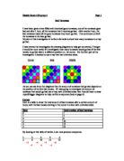
This grid represents the propagation of bad tomatoes in an nxn square, covering grids up to size 24x24. Some of the results for this data are plotted on the table below:
While at first it seems the patterns in this table should be obvious, this is deceptive. Only by splitting the table into three regions do we see the separate patterns defining the table. These regions, as shown in the following table, allow patterns to emerge. These patterns do not, as you would expect, work down with different numbers in the same grids, but instead work across with the same number in different grids.

In the first region (yellow), we see that, in every case, x is equal to n+n-1. The latter two regions (green and purple) are substantially harder, and require a sequential approach. Naturally, the first step in devising a formula, to take n and g and return x, is determining which region the number lies in. This is a simple matter of comparing g with n. Once we know the region, we can use a set op steps to calculate the number x. The method for carrying out this operation will be described shortly.
The left grid shows an updated version of my results ...
This is a preview of the whole essay
In the first region (yellow), we see that, in every case, x is equal to n+n-1. The latter two regions (green and purple) are substantially harder, and require a sequential approach. Naturally, the first step in devising a formula, to take n and g and return x, is determining which region the number lies in. This is a simple matter of comparing g with n. Once we know the region, we can use a set op steps to calculate the number x. The method for carrying out this operation will be described shortly.
The left grid shows an updated version of my results demonstrating the three regions yellow, green and purple, as well as some extra data formulated from the patterns observed. This is the first step in trying to formulate equations to work on all situations. Before moving on to the main essence of the project, finding a formula to derive x from n and g, we shall examine a few other formulae not directly related to this but still relevant to the investigation.
- To find the total number of hours taken for all tomatoes to go bad within a grid, you use a formula depending on g. This formula also depends on whether g is odd or even:
- If g is odd, then h=((g+1)/2)-1
- If g is even then h=(g/2)+1
- In all square grid situations, t is always g2.
- The number of tomatoes to turn each hour in an infinite grid, starting on the side in the centre is equal to 2n-1
- The total number of tomatoes that are bad after each hour is equal to n2.
We shall briefly describe the patterns used to expand this table and in the following formulae:
Yellow numbers always go up by 0 each grid size
Green numbers go up by 1
Purple numbers go up by 3
Green/yellow boundaries go up by 1
Purple/green boundaries go up by 2
We now move on to analyse the main problem: the individual number of tomatoes to turn in each hour. This, as mentioned earlier, is a much more complicated program, and requires division of the grid into three regions. The following steps attempt to demonstrate how, and why, this is done.
- The first step is to compare n with g, to work out which region the answer is likely to lie in. For this example we shall use two numbers, grid size 24 and tomato number 25.
Compare n with g:
If n>g, x lies in the purple region
If n=g, x lies in the green region
If g>n, x lies in green or yellow and further calculation is needed:
If g is odd: if g>= n-((g-1)/2) x is yellow, and if g<n-((g-1)/2) then x is green
If g is even: if g>= n-(g/2) x is yellow, and if g<n-(g/2) x is green
We then move to region specific instructions:
Yellow
x =2n-1
Green
x =g
Purple
(Calculating purple numbers is substantially more complex) (Also note the existence of bln, a new variable we introduce here whose meaning will be explained later)
Do n mod 3:
N mod 3 = 0 then
Bln = 2(n/3)
N mod 3 = 1 then
Bln = (2((n+2)/3))-1
N mod 3 = 2 then
Bln = 2((n+1)/3)
Do g – bln
Again, look at n mod 3:
If 0, multiply last number by 3 and add 1
If 1, multiply last number by 3 and add 2
If 2, multiply last number by 3 and add 3
Therefore, by this process we can calculate any number from the grid size and the hour.
For our example, g = 24 and n = 25, we would do the following:
- n > g, therefore x is purple
- 25 mod 3 is 1, therefore bln = 2(27/3))-1 = 17
- 24 – 17 is 7
- 25 mod 3 is 1, therefore we:
- Multiply 7 by 3 = 21
- And add 2, giving 23
I have checked this with both an extended table of results (created using the patterns found earlier), and with a small excel macro designed to count the numbers of tomatoes turned each hour. Both yield the same result.
The left is the segment from my expanded table showing the result. The ‘23’ in the middle of the table represents grid size 24 and hour 25 – what my formula predicted.
The left here is the automatic count from my macro. The data reads (for a 24x24 table) hour,count (or n,x). This also agrees with my prediction.
We shall here briefly explain how the purple formula works (formulas for both green and yellow are self-explanatory). I observed that the base line (the line marking the bottom of the purple section- representative of the number of tomatoes to turn bad in the final hour) of the purple section follows a three stage recurring pattern. Because we are working from the base line to reach our result, as the numbers go up by 3 each time, calculating the start point and value of the base line for each hour was essential. To work easily with a three -stage recurrence, we needed to work in base 3, the easiest implementation of which involves modulo arithmetic. By doing n mod 3, we work out which stage of the cycle represents the first grid size for tomatoes to turn in a particular hour. Once the cycle is split, we can show different formulae for each stage, derived from observance of the patterns. The variable bln represents the base line grid number- i.e. the grid in which the base line passes through on that hour. Since we know that each grid size increase causes x to jump by 3, we must calculate the difference between the base line and x, in order to work out how many ‘jumps’ we need. This is done by taking the bln(base line grid no) from g, our grid number. We multiply this by three in order to get our number. Finally, we must take into account that the x number on the base line varies on the same three-stage cycle. To do this, we use the modulo function again, to counteract the difference made by the varying numbers. When n mod 3 is 1, the start number is one, and the jumps of three work form this. Therefore, we must add on one each time to take account of this. The same applies for the other stages. In fact, we can shorten the last phase of the operation to
(3(g-bln))+((n mod 3)+2)
Extension
When the bad tomato starts in a corner
Here we have a 20x20 grid showing results for when the original bad tomato starts in the corner of the grid.
The results for this situation are not nearly as complicated as those for when the tomato starts in the middle of a side, and there are only two regions to discuss.
This is the results table for the proceeding grid. As can be clearly seen, there are two distinct regions, red and pink, separated along the line n=g. We can easily see expressions to calculate these:
If g≥n (red) then x = n
If g<n (pink) then x = g+(g-n)
For example, consider g as being 9, and n as being 12. We see that n>g, therefore x is pink. 9 – 12 is –3, and when you add this to 9, you get 6. If we look across the table, we find this is the answer.
We will also try an example out of the range of this table:
Grid size 20 and hour 25. Again, n>g, so we do 20-25. The answer, -5, yields 15 when added to 20, the grid size. By checking this against data extracted by my excel macro, we find this to be the correct answer. The formula can also be expressed more simply as
x = 2g-n
Conclusion
Upon first seeing this investigation, I judged it to be rather uninteresting; my original impression of it was of an oversimplified ‘life genesis’ task. While I still believe the latter to be the case, I have changed my opinion about the former. My original intention was to create a program capable of modelling the propagation of the bad tomatoes automatically, to give me the raw data I would require to find patterns in the data and to create formulae, as I have done. However, it did not take me long to realise I had neither the programming skills nor the tools to do this. I realised later this was not the case; however, by that time there was neither any need for new data or time to create the program. I had to resort to generating data manually, a tedious process. The time it took to generate the data was, I believe, the biggest drawback in this investigation. It took both a lot of drawing and counting to do this, and each different position of the tomato had to be modelled independently. This was why I chose to primarily investigate the effects of changing the grid size; there was no way to effectively find data patterns when moving the first tomato, and it would have taken masses of diagrams. Later I managed to use features in excel to semi-automate the counting and drawing of grids, which helped me to create my final solution, but it would have been helpful for me to have achieved this earlier.
Had I been able, earlier in the project, to create a program to model the spread of bad tomatoes, this would have allowed me to analyse all the data on a much larger and more general scale. While I like to be as general as possible, the sheer amount of data that would have been needed to analyse patterns on a multi-encompassing scale (i.e. to have formulae including starting position and varying side lengths (I.e. rectangular shapes)) made it prohibitive and near impossible to do without an automatic data modelling system. Certainly, were I to have to improve on this project, that would be the first step.
Another drawback of the project was the lack of computer equipment while doing the project in lessons. As I have mentioned, without my automations for the drawing and counting of numbers in a grid, it would have been unlikely that I would have found a pattern. Had I had access to these facilities while doing the bulk of the project, I believe that I would have found the formulae much quicker, and would have gone on to further extend my project, doing such things as look at rectangular grids. As it was, a large amount of time was wasted due to the vast amount of time it would have taken to calculate things manually.
I feel, generally, that the project was a success. Despite a number of setbacks, I was able to find a formula encompassing everything I wished it to, and also did an extension upon the project. Both my main formulae have coped with any numbers I have fed through them, and I have thus far seen no faults in them that were not corrected upon re-examination of the data.