I will use Stratified Sampling to investigate my new hypothesis because it improves the sample by reducing sampling error.
The variables for the sample are gender and age, so I had to do separate samples for boys and girls and vary the amount of samples taken from each year to keep the sample unbiased. This was done as the different year groups had different numbers of pupils and it would be unfair to take the same number of samples from each year group. Therefore, stratified sampling will be helpful due to the fact that there are different numbers of students in each year, and so there is less chance of unequal representation. I will be investigating 20 boys and 20 girls altogether.
I will be calculating my stratified sampling using the table that I have created, and I will now need calculation the proportions of each year to stratify my data.
Stratified Sampling Calculations
I want 40 students from the school total of 1183. Firstly I require 20 boys from the total of 604 boys, and my aim is to work out how many from each year I am going to use. I need to use this equation to do so:
(Number of boys in year ÷ Total number of boys) x Number of boys I require
Year 7 boys = (151 ÷ 604) x 20 = 5
Year 8 boys = (145 ÷ 604) x 20 = 4.8 rounded to 5
Year 9 boys = (118 ÷ 604) x 20 = 3.9 is rounded to 4
Year 10 boys = (106 ÷ 604) x 20 = 3.4 is rounded to 3
Year 11 boys = (84 ÷ 604) x 20 = 2.7 rounded to 3
I then applied the same methods in calculating the number of Girls for my stratified sampling and here is a table of results that I will be using for my data sampling for this particular hypothesis.
Table
Within this process, the decision of choosing students in particular from each year was done via random sampling. This was done by numbering all of the 1183 pieces of data, and then using the “ Ran# ” button on a calculator to randomly select a piece of data. By doing this, and not just picking data randomly myself, I have removed as much bias as possible from this part of my investigation. The results that I collected were typed up on an excel spreadsheet. Since I am only investigating the height and height, I will only show these particular fields in my results.
Stratified Sample Results - Boys
At first, I thought about only putting the heights and weights down, and leaving out the names. However, I realised then that I would have no proof that the data I have come up with is real. Without the names, I would find it difficult to prove that I had not tampered with the data in order to make my hypothesis true. It was acceptable when doing my initial scatter graph because it was initial research to see whether my hypothesis was worth investigating or not.
Stratified Sample Results – Girls
Now that I have my data I will put them into frequency tables because it is a useful way of representing the data and it makes it easier to view trends within the data that I have collected.
Also, I am going to change the height unit from metres (m) to centimetres (cm). I am doing this because it will make it easier to create the frequency tables, and also it will increase the chances of me spotting a trend within the data.
Boys – Height
A pattern I have spotted in this particular frequency table is that nearly 75% of boys are between 150cm and 170cm. This shows me that students in my sample are rather tall, and as it is the majority that are taller, it means that boys of their age are generally tall.
Girls – Height
This table shows me that nearly 50% of female students are between the height of 150cm and 160cm, and there are not many female students who excel over 180cm. Also, there were not many girls with a height between 130cm and 140 cm, which shows me that the spread of data is compact, making it easier to view trends and also it shows that there are not many irregularities in height in the student sample that I have taken.
Comparison
From the sample I have taken, I have found that boys grow rapidly at a later age whereas girls grow faster from an earlier age, and then stop at a particular age. Both girls and boys have average heights, and are fairly balanced / are of equal size. My sample shows that boys on some occasions grow to above average height, such as over 180 cm, whereas in girls this is rare and unique.
Boys – Weight
This frequency table shows the boys weights and the spread of data are large, and not as compact as the height; the heights are rather scattered and varied. This, however, notifies me that some of the students in my sample are tall for their age, but their weights are average in relationship to their height.
Girls – Weight
From this frequency table, I have found that many girls weigh between 40kg and 49kg, and also that hardly any girls weight more than 60kg. This shows me that some girls may stop putting on weight rapidly after a particular age.
Comparison
Most boys and girls from my sample weigh between 40kg and 60kg. I have found that not many girls are over the weight of 60kg, whereas boys are usually borderline 60 or above when they come to the age of 16.
Mean of Frequency Data
I will now calculate the mean of the frequency data that I have found, and this will be quick, efficient and reliable. It will help me to gain evidence on my hypothesis: whether boys are taller and weigh more in comparison to girls.
Frequency Table – Boys Weight
To find the mean from a frequency table, I must use this equation:
Mean = FX ÷ X
Mean = (frequency x midpoint) ÷ frequency
Mean = 980 ÷ 20
Mean = 49
This shows that the mean weight for boys between the years 7 and 11 is 49kg.
Frequency Table – Girls Weight
Mean = FX ÷ X
Mean = (frequency x midpoint) ÷ frequency
Mean = 895 ÷ 20
Mean = 44.75
This shows that the mean weight for girls between the years 7 and 11 is 44.75kg.
Frequency Table – Boys Height
Mean = FX ÷ X
Mean = (frequency x midpoint) ÷ frequency
Mean = 3250 ÷ 20
Mean = 162.5
This shows that the mean height for boys between the years 7 and 11 is 162.5cm.
Frequency Table – Girls Height
Mean = FX ÷ X
Mean = (frequency x midpoint) ÷ frequency
Mean = 3130 ÷ 20
Mean = 156.5
This shows that the mean height for girls between the years 7 and 11 is 156.5cm.
Comparison of Mean of Girls & Boys (Height and Weight)
I have found that, on average, boys are taller and weight more than girls. More specifically, boys weigh around 4kg more than girls, and are taller by about 6cm. This gives strong evidence that my hypothesis is true, and that the boys of Mayfield School are taller and weigh more on average in comparison to females.
Histograms and Frequency Polygons
From the data I have collected and formed through my frequency tables and mean averages, I will now produce a 4 frequency polygons and 4 histograms. I will use boys’ height, boys’ weight, girls’ height and girls’ weight to do this. Both these forms of representing data will help me form a sufficient analysis.
Height – Boys
The following histogram and frequency polygon clearly show to me that the most common height for boys is between 160cm and 169cm, which I believe is average height. This, in my opinion shows that the hypothesis that I have formulated is correct. Although both graphs are representing the same data, I believe that each graph has its value and that both help me to provide a more in-depth analysis and a more accurate conclusion.
Weight – Boys
This particular histogram that I have formed helps me to identify the most common weight group, which you can clearly view from the histogram, and also the frequency polygon. The most common weight is from 40kg to 49 kg for boys, which shows me that this is the average weight for a student studying in the school. Also, I have come to find that no one from the sample that I have taken excels over 79kg, as this polygon clearly expresses, and the trend is also lower in frequency from 40- 49 kg.
Height – Girls
This histogram in particular gives me a clear picture of the data distribution. For the sample I have taken, there is an even distribution of data. The middle group has the highest frequency, which is expected. For the data to be evenly distributed, the other two sides must be fairly symmetrical. It is clear that the histogram does not show this. It shows that the majority of scores were above the median.
This representation of my data shows admirably that the average height is between 150cm and 160cm, which I believe is slightly above average. Personally, also I have noticed that the trend is rather varied, although the frequencies are upward to a certain point and downward from the peak onwards.
Weight - Girls
This data shows that the highest frequency is between 40kg and 49kg. This shows that both boys and girls from the stratified sample that I have taken have a lot In common in terms of frequent data, as the highest frequencies for both are very similar. In addition to this, I have also come to find that the girls do not have many students above 69kg, whereas for boys there are 3 times as many of them above this height.
Cumulative Frequency Diagrams & Tables
I will now produce cumulative frequency diagrams for both girls’ & boys’ height and weight. This will help me gain sufficient evidence towards forming my conclusion. I will also find percentiles and will produce box and whisker plots, as this will help me view my data and trend efficiently.
Height - Boys
Weight – Boys
From this particular cumulative frequency diagram I have been able to find that the average weight from the sample that I have taken is 60kg, which in my opinion is quite high. Also, the inter-quartile range that I will be finding at a later stage will help me view the spread of data and the margin of error. I believe that all the graphs that I will produce will help me complete my objective and conclude efficiently and successfully.
Box and Whisker Plot - Boys Height
Box and Whisker Plot - Boys Weight
Comparison of Box and Whisker Plots
From these box and whisker plots I will be able to find the median, which will show the middle frequency of my data, and also will be able to view the maximum and minimum values for both height and the weight. Then I will be able to find the percentiles and the quartiles.
For the height, the median is 170cm, the inter-quartile range is 30cm, the maximum value is 200cm and minimum value is 140cm. For the weight, I have found the median as 60kg. This is respectively what I had predicted and is suitably accurate, although the range of data for the weight is less and the data is negatively distorted in comparison to the height for the boys.
I will now be producing cumulative frequency tables and a diagram for the girls’ height and weight, since this will help me form a sufficient and reliable comparison in height between girls and boys, and in turn form a successful and accurate conclusion to my hypothesis.
Height – Girls
On this cumulative frequency diagram I have labelled the median, but also the upper and lower quartile. Through this, I will find the spread of data and also the middle number of the data of girls’ heights. The median for this graph is 165cm, and the inter-quartile range is: 177cm – 154cm = 33cm. These discoveries will help toward my final analysis.
Weight – Girls
On this cumulative frequency diagram I have labelled the median, but also the upper and lower quartile. Through this, I will find the spread of data and also the middle number of the data of girls’ heights. The median for this graph is 60kg, and the inter-quartile range is: 70kg – 50kg = 20kg. These discoveries will help toward my final analysis.
Comparison of Height and Weight of Boys and Girls from Cumulative Frequency Diagrams and Box Plots
From the cumulative frequency diagrams, I have come to find that the median height for boys in the sample that I have taken is larger in comparison to the girl’s median height; the boys median height is 170cm, whereas the girls median height is 162cm. This shows that there is an 8cm difference in the middle figure from both sets of data I have collected. Also, the range of data varies, as the inter-quartile range for boys is 21cm and for girls it is 33cm, which shows that the spread of data that I have from my sample for boys is narrower; girls have a wider spread range. This makes the results more reliable as a whole. As far as the weights are concerned the range is similar, and even rather symmetrical.
Evaluation of Hypothesis
In my honest opinion, I feel that I successfully completed and analyzed my hypothesis and have gained a sufficient evidence to back up my theories. I would like to remind you that my main objective for this hypothesis was to find out whether I was correct or incorrect in my thinking that boys at Mayfield School are taller and weigh more on average than the girls at the same school. Within this aim, I was also aiming to find whether there is a certain trend or relationship between the height and weight of the students that I have chosen to analyse. Also, as I explained earlier, due to the large number of students I was unable analyse all students. Therefore, I gained a sufficient sample which I made as unbiased as possible, and got my results from the pieces of data that I randomly collected.
Conclusion of Hypothesis
- The histograms and frequency polygons proved that the results were more accurate, and made more sense than that from the random sampling.
- There is a positive correlation between height and weight. In general, tall people will weigh more than smaller people.
- In general, boys tend to weigh more and be taller than girls.
- By doing stratified sampling, there were fewer exceptional values caused by different year groups and, therefore, ages. I was bound to find irregularities within my data from the start.
- The cumulative frequency curves confirm that boys have a more spread out range in weight, with more girls having smaller weights. In height, boys tend to be taller.
- In general the taller a person is, the more they will weigh.
- There is a positive correlation between height and weight across the school as a whole. This correlation seems to be stronger when separate genders are considered.
- If I had taken larger samples my hypothesis may become more accurate.