Secondary Data
When I was researching into possible sources of data, I was told that data that had been collected about students at a secondary school was available. When I looked at the data, I realised that there were enough observations for me to be ale to carry out a meaning investigation. In particular, the data was available in raw format. In other words, I did not need to worry about the data having been previously manipulated.
Hypotheses
1. Distribution
1.a. The distribution of the heights and the weights will be approximately normal
1.b. The spread of the girl’s heights will be more than the boys’.
2. Comparative
2.a. On average, the boys will be heavier than the girls
2.b. On average, the girls will be taller than the boys
2.c. As the height increases, the weights will increase I proportion.
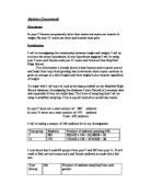
Methods
Data Collection
The data that I got from the school contained a great deal of information about the pupils, including their IQ, their examination results, their dates of birth and the subjects that they studied.
I decided to investigate height and weight because I expect to find some kind of relationship between the two and since these are parametric data, I will be able to do correlation analysis also.
Choosing the Data
Stratified Sampling
There were 119 boys and 143 girls in the year 9 group. I felt that this was too many and I decided to use stratified sampling to collect a representative sample.
I decided to work on a total of 80 pupils and calculated the number I need from each group by multiplying the proportion of each sex from the total by 80. i.e.
Boys’ sample: (boys/total)x80
Girls’ sample: (girls/total)x80
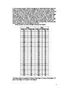
The able below shows how many pupils I chose from each group:
Randomised Selection
After finding the number of pupils that I would need from each group, I used the Rand() function in Excel to generate a random number for each set of data. I then sorted the data by that column and selected the first 36 for the boys and the first 44 for the girls.
Testing the Hypotheses
Analysis and Interpretation of Data
Data Summaries
From the above statistics, box plots can be drawn. These will give a general comparison of the spread of the data and will allow limited comparisons to be made between the data.
Measures of Spread of Data
Box and Whisker Diagrams
A comparison of the Box Plots for Boys and Girls’ height indicates that the boys’ height distribution is more skewed than the girls. The interquartile ranges also indicate that there is a greater spread of heights amongst main body of girls, whilst most of the boys are bunched up within a narrower band indicating that there may be a few ourtliers in the boys’ population.
A comparison of the Box Plots for Boys and Girls’ weight indicates that whilst there is a greater spread amongst the girls, the distributions are more comparable than with the heights.
Stem and leaf and Frequency Table (Boys Height)
This distribution can be seen more easily by drawing a graph:
From the look of this graph, it can be assumed that the distribution of boys’ heights is ‘normal’.
Stem and leaf and Frequency Table (Girls Height)
This distribution can be seen more easily by drawing a graph:
From the look of this graph, it can be assumed that the distribution of girls’ heights is skewed. The skew is much more noticeable from this graph than from Box Plots.
Stem and leaf and Frequency Table (Boys Weight)
This distribution can be seen more easily by drawing a graph:
This graph looks slightly skewed, but there are too few data at the periphery of the distribution to be sure.
Stem and leaf and Frequency Table (Girls Weight)
This distribution can be seen more easily by drawing a graph:
From the look of this graph, it can be assumed that the distribution of boys’ weights is ‘normal’ since a single data point moving from the 55 to 45 would make the distribution symmetrical.
Standard deviation and confidence intervals
95% Confidence intervals*
The 95% Confidence intervals indicate that there is a 95% chance that samples from this population will fall within the two intervals.
Comparing heights against Weight for Boys
Correlation Analysis
The results of the correlation analysis (see graph inset) gave an r-squared value of 0.15. This means that only 15% of the variation in weight can be attributed to the variation in height.
Comparing heights against Weight for Girls
Correlation Analysis
The results of the correlation analysis (see graph inset) gave an r-squared value of 0.038. This means that only 3.8% of the variation in weight can be attributed to the variation in height.
Conclusions
Hypothesis 1.a.
The distribution of the heights and the weights will be approximately normal
With the exception of the girls heights, there is strong indication that this is true.
Hypothesis 1.b.
The spread of the girl’s heights will be more than the boys’.
The results showed that this hypothesis is not true.
Hypothesis 2.a.
On average, the boys will be heavier than the girls
The analysis indicates that this hypothesis was not true.
Hypothesis 2.b.
On average, the girls will be taller than the boys
This was also shown not to be true.
Hypothesis 2.c.
As the height increases, the weights will increase in proportion.
Although there seems to be a slight linear relationship, there is too much variability in the data and for boys, only 15% of the variability can be attributed to the variability in weight can be attributed to height and for girls, this becomes even less at almost 4%.
Evaluation
Overall, the results for the comparison of heights and weights were surprising. I expected to see a much greater relationship between height and weight and a greater difference between boys and girls.
However, the distributions were as I expected.
If I were to do this project again, I would do the analysis taking account of the outliers.
Appendix 1 – The data