To find a correlation, the top left and bottom right quadrants (1 and 3) have to be compared with the bottom left and the top right quadrants (2 and 4), in terms of the number of points they have all together. I think that I will see that there are more points in quadrants 1 and 3 than in quadrants 2 and 4, making it a negative correlation. If 2 and 4 had the most points it would be a positive correlation. I think that my graph will have a negative correlation because 1st place in the house run is at the left
Hypothesis 2:
I predict that as pupils go higher up the school; their bleep test scores will be higher.
I think this will happen because as you grow up, your fitness and stamina increases, making you able to run for a longer period of time. Also, the higher up you go in school the more experience you have of training and fitness and therefore, you are likely to do better than when you were younger.
I will investigate this hypothesis by using box plots. I will first take out any data that I cannot use or that is incomplete. I will use the Y10 class 3 bleep test history spreadsheet that I have been provided with from the shared area. This spreadsheet shows the bleep test scores of a year 10 class from year 7 to year 10. I will take the autumn bleep test scores of the pupils from each year they did the test in. I will need to sort all of the pupils’ information into ascending order. This will give me my lowest and highest values. Then, by using Excel, I will be able to find the lower quartile, upper quartile and median as well as the mode.
Box plots are useful for comparing the mean and median scores of the bleep test as well as finding out the skewness. The skewness is like the correlation but of a set of box plots. It also shows additional information such as the lower and upper quartiles. All of this information will help me interpret my results.
In order to predict what I will see in terms of the skewness of the box plots I have made two stem and leaf diagrams: 1 for the pupils’ year 7 bleep test scores, and 1 for the pupils’ year 10 bleep test scores. This will help me compare the 2 and look for any particular shape that takes place. I have done this on Excel by sorting the data in ascending order and then taking the information to make a stem and leaf diagram.
As shown here, the year 7 diagram has most of the information near the top and the highest value is at the score: 10. But the year 10 diagram shows that most of the information is near the bottom, showing higher scores in the bleep test: 12. These diagrams show that the year ten scores are better than the year 7 scores, which helps me see what the box plots results will look like.
A set of box plots and take the form of 3 appearances. These appearances are the skewness: a measure of which end of the data most values lie. There is positive skewness- when the median is lower than the mean; negative skewness- when the median is higher than the mean; and symmetrical skewness- when the median and the mean are the same.
I think that I will see both positive and negative skewness; positive in Years 7 and 8, but negative in Years 9 and 10. I think this because as pupils go higher up the school, more and more get higher than the mean, and those who get less decrease the mean.
I think that my box plot will look like this, showing both positive and negative skewness. The method of finding the skewness will consist of me making comparisons between the mean and median values, which will help distribute my data correctly.
Using a set of box plots for this hypothesis is very useful because it handles with discrete data and helps compare the distribution of that data. It also helps in comparing the different box plots as well as their skewness.
Hypothesis 3:
I predict that the Year 10 rugby team players will get a higher bleep test score than those pupil’s who aren’t in a school team.
I think this because being in a school team, such as the rugby team, encourages physical training. Pupil’s who are not in a school team are less likely to get a high bleep test score because they might not do any physical training in school, but they might be doing physical activities outside school.
To investigate this hypothesis I will use the Yr 10 data spreadsheet provided from the shared area. First, I will have to delete any data that I cannot use, such as the data of pupils that were absent during the spring bleep test, as well as the data of pupils that are in the school rowing team, as my hypothesis only requires the data of rugby players and pupils in no school team.
After I have all the data I need, I will need to sort my day so that I have the information of rugby and non-rugby players. However, there are many more non-rugby players than rugby players, which means that I will need to fairly take the same amount of non-rugby players and rugby players. I plan to take all the rugby players in Year 10 and use the randomising method on Excel, like I did for Hypothesis 1.
Next, I will need to make a table showing the cumulative frequency. This will consist of the bleep test score in one column, the frequency of that in the other, and an extra column showing the cumulative frequency.
Once I have the same amount of non-rugby players and rugby players, fairly taken by using the randomising method and the plots taken from the table, I will use cumulative frequency graphs to interpret my results. Cumulative frequency is used to compare the distribution of two sets of data, which is why it is so relevant to my hypothesis. They also help in calculating medians and quartiles easily as well as data above and 10% within the average. Proportions of data in given ranges can also be calculated easily using cumulative frequency graphs, such as the data between bleep test scores 7 and 10.
I think that my cumulative frequency graph will look like this, showing that the rugby players get a higher bleep test scores than the non-rugby players. Also, the rugby players’ scores will be more bunched up together and the amount of scores in the range of within 10%of the median will be much higher in the rugby players’ curve than in the non-rugby players’ curve, which will be more spread out.
To further compare my two curves, I will need to look at the measure of central tendency as well as the measure of central dispersion. The measure of central tendency will help me compare points on the curves, such as the mean, median and the mode of the data. The measure of central dispersion looks at the spread of data, such as the range and quartiles.
The red curve shows the rugby players’ curve.
The black curve shows the non-rugby players’ curve.
Plan Overview:
Hypothesis 1: I predict that the better the pupil’s position in the Pe house run, the higher the pupil’s spring bleep test score
Hypothesis 2: I predict that as pupils go higher up the school; their bleep test scores will be higher.
Hypothesis 3: I predict that the Year 10 rugby team players will get a higher bleep test score than those pupil’s who aren’t in a school team.
Hypothesis 1 Hypothesis 2 Hypothesis 3
I think that this will be my three sets of results by the end of my investigations.
Analysis
Hypothesis 1: For this hypothesis I used the 4 year data spreadsheets of Years 7, 8, 9 and 10. First I took any data that I could not use, such as the data of pupil’s who did not run, were absent or were injured. I also deleted the information showing what School Team the pupils were in, what level they were at on their musical instruments and also the Pe autumn bleep test score, as I was not going to be needing these pieces of data. However, classes 2 and 3 of year 10 had not done their bleep test in spring, so I took their autumn bleep test score, to make up for the missing gap.
After deleting all the unwanted data for every year group I had to use the method of Stratified Random Sampling to obtain the number of pupil’s information I will need to use from every year group.
First I took the total number of pupil in the year (after incomplete data had been deleted) which was 463. I also took the total number of pupils in each year group and I end up with this:
Year 7: 107 Year 8: 119
Year 9: 127 Year 10: 110
I then used the Stratified Random Sampling method which consisted of me doing the following:
Year 7: 107/463 x 40 = 9 (no d.p)
Year 8: 119/463 x 40 = 10 (no d.p)
Year 9: 127/463 x 40 = 11 (no d.p)
Year 10:110/463 x 40 = 10 (no d.p)
This method gave me the number of pupils I have to take from each year for this investigation. But there are over 100 pupils in each year, and I have to take only 9, 10 or 11 of them. To do this fairly, I used another randomising method on Excel. I put in the formula: =RAND( ) and got a random number. Then I dragged that cell down to the end of my data, giving me a column of random numbers. Then I copied these columns and used special paste, so that the random numbers do not change. Finally I sorted those numbers into ascending data, which left me with my randomised data. I then took the number of pupils I needed from each year from the top, giving me the final data I needed. My final data consisted of a certain number of information from each, fairly obtained by randomising using Excel. I then used this data to draw my scatter graph.
Hypothesis 2:
I used the Year 10 class 3 bleep test history spreadsheet to investigate this hypothesis. In order to make my set of box plots I must process the data. First, I took out the pupils who were absent as well as the spring bleep test scores which I was not intending to use. Then I took copied and pasted all the columns with different year bleep test scores separately, with the pupil numbers next to each one. Then I sorted each column into ascending order. This gave me 8 columns: 4 for the different year bleep test scores and next to each one was the pupil numbers column, as shown below:
This piece of data helped me make my stem and leaf diagrams for the bleep test scores of the pupils when they were in Year 7 and when they were in Year 10. This piece of data will help now me obtain the highest and lowest value, lower and upper quartiles and the mean, median and mode, all done with the help of excel.
To find the quartiles and values I used Excel: I inputted the formula =QUARTILE(highlighted data, quartile number). I highlighted the column of each year separately and then put in a certain quartile number, which gave a certain value.
Quartile numbers:
Lower Quartile: 1
Median: 2
Upper Quartile: 3
To find the lowest and highest values of each column I simply took the top and bottom numbers of the columns. To find the mean/average and the mode, I used the formulae: =AVERAGE(data) and =MODE(data). This then left me with the diagram below.
After I had got this information I used these values to draw my set of box plots and interpreted them.
Hypothesis 3:
For this hypothesis I used the Yr 10 data spreadsheet provided from the shared area. First, I deleted all the data I could not use, such as the data of pupils who were absent, injured or who were in the school rowing team. I deleted the pupils in the rowing team because they undergo a lot of physical exercises and do not support my hypothesis. Then I sorted my data so that I had the rugby players at the top and the non-rugby players underneath. I found that in total there were 34 rugby players, which meant that I needed to get 34 non-rugby players.
To do this fairly, I used randomising on Excel, just like I used in hypothesis 1. I typed in the formula ‘=rand()’ and I got a random number. I dragged the cell down until it covered all the data of the non-rugby players and then I copied it and selected ‘paste special’. A window then came up asking what I want to keep the same; I selected values and all the values were set. I then sorted the data again to give me randomised data of the non-rugby players. (This process is shown on the previous page). This allowed me to take 34 non-rugby players fairly and get all the information I needed to make my cumulative frequency table.
My frequency table gave me the points that I needed to plot in my cumulative frequency graph, giving me the two curve and my results. Then, I used Excel again in order to obtain the mean, medians and quartiles of both curves, this gave me the measure of central tendency- looking at points on the graph. From the quartiles I could see the inter quartile range, which gave me the measure of central dispersion- looking at the spread of data.
All of this information that I have acquired will help me in interpreting my results.
Results
On the next three pages are the three graphs that I drew after planning and analysing each hypothesis. First there is the scatter graph, then the set of box plots, and finally the cumulative frequency graph. I will interpret these graphs in order to see whether or not my hypothesis were correct or incorrect and also explain why they were like this.
Interpreting the results will also help in comparing different aspects of the graph.
In the end, this will lead to a conclusion which will end the investigation for the hypothesis.
Interpretation
Hypothesis 1:
My results show a scatter graph linked to my hypothesis. Overall, my prediction - that the better the pupil’s position in the Pe house run, the higher the pupil’s spring bleep test score – was correct. As shown on the scatter graph, there was a negative correlation that I had expected. It showed that the points that were higher up the graph were also more to the left, showing that the higher the bleep test score, the better the position in the Pe house run.
The negative correlation is shown by the number of points in each quadrant of the scatter graph:
Quadrant 1: 23
Quadrant 2: 5
Quadrant 3: 8
Quadrant 4: 4
This shows that quadrants 1 and 3 had more points than quadrants 2 and 4. Also, most of the points were in quadrant 1, but there are some points that do not match my hypothesis. For example, in quadrant 1 there is a pupil who came second in the Pe house run and got 11.2 in his bleep test, but another pupil who came seventh got 12.6 in his bleep test score. This shows that using all 4 year groups may not be as effective as doing all 4 year groups separately, which is what I shall consider if I continue to investigate this hypothesis.
On the scatter graph I have also drawn a line of best fit. It is no very steep, but it still shows that when it runs though the point where the means of the axis meet, both ends of it are in quadrants 1 and 3. This also enforces my findings of a negative correlation which I predicted to see.
For this hypothesis, my prediction is proven correct by the scatter graph.
Hypothesis 2:
My results show a set of box plots that are linked to my hypothesis, but there is an area that I did not expect. Overall however, my prediction - as the pupils go higher up in the school, their bleep test score increases - was correct. As shown on the box plots, the box plots go higher up the scale as the year increases. Also, the range between the lower quartile and upper quartile decreases, showing that the pupils were more consistent and more pupils got higher scores like everyone else in their age group.
The box plots show that the Year 7 scores had a big range between the lower quartile (Q1) and the upper quartile (Q3). This shows that the pupils got very different scores to each other, some got extremely low and others got very high scores. The median (Q2) was also quite low.
The box plots show something that I did not expect it to show for the Year 8 scores. It shows that the Year 8 pupils got the lowest score, as well as almost the same highest score as the one in Year 7. However, the range between Q1 and Q3 is lower than that of the Year 7 scores, which I predicted I would see. Also the Q2 is higher, showing that the Year 8 scores were better than the Year 7 scores.
The box plots show that the Year 9 scores have a higher score than the Year 8 and Year 7 scores. It also has a smaller range from the highest and lowest scores, showing that more pupils were getting higher scores. The range between Q1 and Q3 is also quite small; smaller than both Year 7 and Year 8 and Q2 is also higher than Years 7 and 8, showing that the Year 9 scores were better.
The box plots show that the Year 10 scores are overall the best scores out of all the other Year scores. The Year 10 pupils have got that highest bleep test score and also the best lowest score. The range between Q1 and Q3 is roughly the same as that of the Year 9. However, the Year 10 median is very high, showing that most pupils got very high scores. Overall, Year 10 had the best bleep test results, but Year 7 had the worst.
Looking at the medians of each Year score shows the improvements or loss in the bleep test score of the pupils throughout the 4 years:
Year 7: 6.5
Year 8: 7.5
Year 9: 8.5
Year 10: 9.7
The medians show that there is a big increase in the
To work out the skewness of this set of box plots I looked at the link between the median and the mean:
Positive: Median < Mean
Symmetrical: Median=Mean
Negative: Median > Mean
As shown in the table above, each year group has a negative correlation, as the medians are higher than the means. My prediction was that I will see both negative and positive skewness, however that is not the case. This might have to do with the fact that as the pupils go higher up the school, the position of the box on the scale increases and the inter quartile range in the box plots decreases, therefore the data is less spread out. If the data is less spread out, the than the mean should go higher and higher, and it does, but not high enough to show positive skewness.
This shows that as the pupils go higher up the school; their bleep test scores are higher, proving that my prediction was correct.
Hypothesis 3:
My results show that the cumulative frequency graph is linked to my hypothesis. Overall, my prediction - I predict that the Year 10 rugby team players will get a higher bleep test score than those pupil’s who aren’t in a school team – was correct. As shown in the cumulative frequency graph, the rugby players’ curve is further to the right than the non-rugby players score, showing that they got higher bleep test score. Also the rugby players’ line is much steeper than the non-rugby players’ line, which shows that the spread of data is more for the non-rugby players.
On the whole, the cumulative frequency graph’s shape was the same as my prediction. It shows that the non-rugby line is very inconsistent and moves up and down, it also has a very steep line between the LQ and the median. Whereas the rugby players line is very consistent as it is smooth and there are no harsh turns in the line. This shows that the rugby players achieve much more consistent scores than the non rugby players, who get a very big range of scores. This might be due to the fact that there were many more non-rugby players than rugby players, which means that the range will be big. In order to achieve the best results, I will need to get a spreadsheet only showing one class with many rugby players, to lessen the amount of non rugby and maybe obtain a more accurate result.
On the cumulative frequency graph, the quartiles drawn show a clear finding of this investigation. The lines labelled with a red pen show the quartiles and median for the rugby players. The lines labelled with black show the non-rugby players. The lower quartile of the rugby players is higher than that of the non-rugby players. The upper quartile of the rugby players is lower than that of the non-rugby players. The inter quartile range (IQR) is equal to UQ – LQ.
RUGBY: UQ – LQ = 11.5 – 9.8 = 1.7 13.5(cf)
NON- RUGBY: UQ – LQ = 9.6 – 7.2 = 2.4 20(cf)
This clearly shows that the rugby players’ scores are more consistent than the non-rugby players, which are widely spread out which is what I predicted to see.
This shows that rugby players get better bleep test scores than non-rugby players, proving my prediction correct