Results: N.B. All Prices are in £, all ages in years and depreciation in percentages.
These are my Graphs for Colour against Price:
Colour against Price:
As you can see, the scatter graph shows little evidence for a possible correlation and this proves that the colour of the car has minute effects on the price.
Engine Size against Price:
As you can see there is one point in this scatter graph which has caused the graph to look wrong and this point belongs to the Peugeot Graduate which, instead of being listed normally, the engine size has been listed in cylinder size. After using secondary sources such as the internet I have discovered that this 1989 Graduate had an engine size of 1.1 and if I change that result this is the graph I am left with:
Through this graph, we can see a weak but positive correlation which proves my prediction to be correct. I shall now try to use only a certain model which should eliminate those outliers from cars which had an expensive original price or those which have lost value much faster than the others.
Using just Fords, I have made a scatter graph to show how much more the sample has been refined and how much stronger the correlation gets when you refine the sample, without any proper outliers, this graph has a positive correlation.
Although this graph has a strongish correlation I do not believe that this is relevant because it uses the 2nd hand price which will be largely subject to the age rather than the engine size, I believe it would be more relevant if I took the original prices against engine size and than used the depreciation to relate it to the 2nd hand price.
Again by using just Fords, I have made a graph which clearly shows a positive correlation but there are too many outliers to make a formula. So I would need to choose a specific model to try to make a formula.
Age against Price:
Using all 100 cars I have drawn a scatter graph for the age against price and because it is obvious that there is a negative correlation, I have decided to draw a trend line. As you can see there are three main outliers and one which is a possible outlier to the pattern and these are caused by cars with a higher original cost so if we were to use percentage depreciation against price we should have a stronger correlation. But first I shall use specific models to produce graphs in order to form some formulas.
In the overall age against price graph there were deviations from the trend line of up to £12000 compared with the maximum deviation(difference) of about £3000 which proves that this graph has a much stronger correlation which is of course positive.
I shall now compare this graph to that of another make's.
This graph is about 4 times stronger than the overall graph but the maximum deviation from the trend line reaches about £3000, so it is has as strong a correlation of the Ford's Graph.
It would seem that the Fords in my sample generally lose value faster than Rovers judging by the trend line, (Rover's trend line reaches slightly below 2000 after about 7 years compared to the Ford's trend line reaching 2000 in about 6 years) but this may be due to lower original prices. I did decide to look at this and found that the average original price for Fords in the sample is £11319.75 and Rovers average is £15813.55 which could prove that this information is irrelevant
I shall now calculate formulas for both trend lines so we can have an idea of how much a car should cost after it is χ years old.
To calculate the gradient of the trend line I must take two points from the line, and because the trend line is a straight line, the formula should look something like y=mx+c,
The points I have chosen from the Fords graph are (2,8000) and (4,5000).
So Price = -1500 × Age + ?
-1500 × 2 = -3000 8000 - -3000 = 11000
So Price of 2nd hand Fords = -1500 × Age + 11000
Example: -1500 × 4 = -6000 -6000 + 11000 = 5000
And my formula works.
Using the same method I worked out the formula for the Rovers using the points (2, 12000) and (6, 3700) which came to:
Price of 2nd hand Rover = -2075 × Age + 16150
Following my comparison of the graphs this shows that it was in fact wrong as the gradient of the trend line of the Rovers is negatively steeper than that of the Fords which proves that for my sample Rovers lose value faster than Fords but have a higher original value.
I shall look at percentage depreciation.
I have used this formula to work out the percentage depreciation:
There is only one real outlier in this graph and that belongs to the 15 year old Volkswagon Golf. The computer sets the depreciation for this car as 0 because there is no recorded value for the original price of the car in the spreadsheet.
I shall now refine my results and calculate average yearly depreciation for specific makes such as Ford or Vauxhall.
This graph has a stronger correlation than the overall graph, this is because it has been refined and the average depreciation per year is about 5% per year after the 1st year.
This graph of age against percentage price depreciation for Vauxhalls has a slightly weaker correlation than the one for Fords and from it we can see that generally Vauxhalls lose value at about 7% per year, but I shall now be calculating the actual depreciation per year by working out the formulas for the trend lines. The gradient in these formulas or the m in y=mx+c will be the number which is multiplied by the age and will be the percentage depreciation per year for the trend line. Also c is the depreciation of the car which occurs immediately after it has become a 2nd hand car.
Fords: Using the same method as I used before I have acquired the formula, Percentage Depreciation = 5 × Age + 35 so the depreciation per year is about 5%. Also Fords lose 35% of their value after they have been used.
Vauxhalls: Again I shall use the same method to acquire the formula, Percentage Depreciation = 7.5 ×Age + 22.5 so the depreciation per year is about 7.5% and Vauxhalls lose 22.5% of their value after they have been used.
Conclusion:
From this investigation, I have found that the price is mainly affected by the age and original price of the car although the make, model and peripherals also affect the price although they affect the original price which in turn affects the 2nd hand price. I am now also able to find out which cars lose value faster and I am also able to apply this in a business if I were to choose such a profession.
Although I was unable to use secondary sources because of information which was not included in the information (mainly original price), I was still able to use information in the sample I had to refine my graphs so I could have definite results. I have learnt many things from this investigation, mainly what affects the price of 2nd hand cars most and this may in future influence my choice of car which I plan on buying.