PIE CHART: The pie charts will be used to show the relationship between height and age group. The result will then compared between boys and girls of the different age groups.
11 – 14 years: Male Female
15 – 16 years: Male Female
20+ Male Female
With reference to table 1, the median group and estimated mean in the sample were higher for boys than for girls. However the sample for girls in year group 7-9 were more spread out with a range of 0.49m compared to 0.39m for the boys. This must have affected the mean. The evidence from the sample suggests that in year group 7-9, 12 boys out of 41 pupils, have a height between 1.6m and 1.69m whilst 7 girls out of the same 41 pupils have a height of 1.6m and 1.69m. This prove that the first part of my hypothesis is wrong: i predicted that in year 7-9, more girls would be taller than boys but my result shows more boys to be taller than girls.
However in year group 10-11, there were more girls than boys with a height between 1.6m and 1.69m though the samples for boys were more spread out with a range of 0.49m compared to 0.39 for the girls. Once again my hypothesis is wrong because i predicted that in year 10-11, boys would be taller than girl.
These conclusions are based on a sample of only 60 pupils. Therefore the limitation of data could have affected the accuracy of my hypothesis. If I could extend the sample my hypothesis is likely to be right.
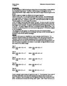
MEASURES OF AVERAGES
Heights
Year group 7 - 9: Male Female
Estimated mean = 34.045 = 31.52
21 20
= 1.62 = 1.57
Year group 10 - 11 Male Female
Estimated mean = 15.305 = 16.65
9 10
= 1.70 = 1.67
20+ Male Female
Estimated mean = 16.55 = 17.452
10 10
= 1.66 = 1.75
Table 1
Measures of average: heights (metres)
CUMULATIVE FREQUENCY: the cumulative frequency graph will be used to compare the boys and girls weight in each age group. I will be commenting on the inter-quartile range and median and making reference to the box plot.
Year group 7-9 Male Female
Year group 10 - 11: Male Female
20+ Male Female
All three measures of average (mean, median and mode) are similar for boys and girls in year group 7-9. The sample on boys has a mean of 49.7kg while girls have a mean of 49kg. However the range shows that the boys sample are more spread out with a range of 59kg unlike that of girls with a range of 39kg. The box plot shows the inter-quartile range for both boys and girls to be similar. This suggests that their weights are within the same spread. The modal group for boys and girls are the same which tells that majority of boys and girls I sampled weight the same. With reference to my hypothesis, the results show that it is wrong. I predicted that boys would weigh more than girls but the results suggest that their weights are similar.
The weights for year group 10-11 prove my hypothesis right. The mean as a measure of average is higher for boys than for girls. Table 3 shows the estimated mean for boys to be 58.9kg and 50.5kg for girls. The box plot shows that the girls’ inter-quartile range is 4.6kg less than the boys’. This suggests that the boys’ weights are more spread out than the girls. Evidence from table 2 shows the maximum value for boys to be 89kg whereas the maximum value for girls’ is 69kg. However the boys sample has a bimodal distribution.
As for the adult data, all three measures of average are greater for the men than for the women. However, the range is greater for women than for men. The box plot shows the inter-quartile range for women to be 29.8lg while that of the men is 15kg. This suggests that the women’s sample was more spread apart than that of me. Table 3 shows that the women’s sample has a range of 59kg while the men’s sample has a range of 29. However the estimated mean shows the men to be heavier than the women with an estimated mean of 82.5kg in comparison to the women’s estimated mean which is 59kg. The adult data supports my hypothesis and proves that it is right.
Table 2
Weights
11 – 14 years Male Female
Estimated mean = 1044 = 980
- 20
= 49.7 = 49
15 – 16 years Male Female
Estimated mean = 530.5 = 505
9 10
= 58.9 = 50.5
20+ Male Female
Estimated mean = 825 = 665
10 10
= 82.5 = 66.5
Table 3
Measures of average: weight (kg)
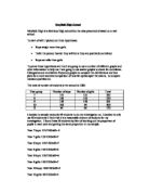
Histogram
Year 7-11 Male Female
61% of the sample appeared to be underweight: 33% being boys’ and 28% being girls’. This is seen from the histogram drawn for year group 7-11, which proves that my prediction is right. The female BMI data is closer to its mean in comparison to the boys’ data. Evidence from table suggests this. A standard deviation of 2.48 tells how close each BMI value is to the mean in comparison to the boys’ standard deviation of 4.05 which suggests that each data is more spread out from the mean (19.49). I also predicted that most of the girls would be overweight. However this was not the case: 5% of boys in the sample were overweight with no girl being overweight. This could have been as a result of limited data as this sample was based on only 60 pupils out of a possible 1183. If I were to extend my sample, then my hypothesis is likely to be correct.
Standard Deviation
Year group 7-11
Male female
SD = √ ∑ x2 – x2 SD = √ ∑ x2 – x2
n n
= √ 396.267 – (19.49)2 = √ 377.374 – (19.26…)2
= √ 16.4069 = √ 6.1695…
= 4.05 (2d.p) = 2.48 (2d.p)
20+ Male Female
SD = √ ∑ x2 – x2 SD = √ ∑ x2 – x2
n n
= √ 625.963 – (24.89)2 = √ 617.011 – (24.39)2
= √ 6.4509 = √ 22.1389
= 2.54 (2d.p) = 4.71 (2d.p)
The standard deviation of the national data is smaller than that obtained from my investigation. This tells that my values are more spread out. However the standard deviation of the national data was derived from a large sample in comparison to mine.
My sample was based on only 20 adults aged 20 and over and the oldest in my sample was aged 56. Therefore the data was limited; whereas the national data was based on 3,625 adults aged 16 and over.
Due to a limitation of data, my values are not very close to the mean in comparison to that of the national data. The standard deviation of male adults is 2.54 and that of the female is 4.71. These figures tell how close the values are to the mean and from table 5 (above); we can tell that the male data is closer to its mean of 24.89 in comparison to the female data with mean of 24.39.
In contrast to my data, the standard deviation of male and female data from the national data for 2002 is 0.08 and 0.09, respectively. This tells that the values are very close to its mean of 26.9 and 26.7.
Summary of National survey
The Health Survey for England carried out in 2002 focused on the health of children and young people, and on the health of infants, aged under one, and their mothers. The survey showed that 16% of boys and girls aged 2 – 15 are obese and almost 30% are either overweight or obese. This is because the rate at which the children aged 8-15 smoke has increased from 1995 to 2002. In 1995, roughly 22% of boys and girls did not smoke compared to 19% of boys and girls that do smoke now. This has resulted to obesity and low fruit and vegetable consumption.
Although more women eat five or more portions of fruit than men, it appears that the percentage of overweight or obese women is higher than that of men. The survey shows that 33% of young women are either obese or overweight whereas 32% of young men are either overweight or obese. Almost 9% of young men and 12% of young women are actually obese.
More women are overweight and obese because they eat to respond to their problems. Information from the survey shows that 52% of mothers from lone parent households said they felt they did not have much social support. This is twice as many as in two parent households (23%). In the same way, women respond to their problems by smoking. The survey showed that 33% of men and 35% of women currently smoke cigarettes. The percentage of women is more than that of men because more women said they did not have much social support. The same applies to alcohol consumption. The proportion of young women who drink more than the recommended weekly limit has gone up by a half in the last five years. The survey shows that in 1997 just over 22% of young women reported drinking more than the recommended limit of 14 units of alcohol in a week. The latest figures, from 2002, showed that almost 32% were drinking over the recommended limit.
Conclusion
The investigation did prove some of my hypothesis right. However some were not proved right. This must have been the data was limited by sampling only 60 pupils out of a possible 1183 pupils at Mayfield high school.
- A sample of 60 students stratified over age and gender shows a mean height of 1.6m for boys and 1.57m for girls in year group 7-9 and 1.7m for boys and 1.67m for girls in year 10-11. This shows that boys in the sample are taller than girls. The data on table 1 shows that most of the boys have a height between 1.6m and 1.69m; with 1 boy having a height of 1.9-1.99m.
The adult data does not prove my hypothesis right. All three measure of average in the sample are higher for the females than for the males, though the sample of males were more spread out with a range of 0.29m compared to 0.19m for the females. This suggests that the women in the adult sample are relatively taller than the men.
- All three measures of average are higher for boys than for girls. In year group 7-9 the median and mode as a measure of average was similar. However, the data shows that boys weight more than girls in the same age group. Table 3 shows the estimated mean for boys in year group 10-11 to be 58.9kg and 50.5kg for girls in the same year group. The box plot shows that the girls’ inter-quartile range is 4.6kg less than the boys’. This suggests that the boys’ weights are more spread out than the girls. As for the adults all three measures of average are greater for the men than for the women. The adult data supports my hypothesis and proves that it is right.
- There is no correlation between body mass index and age both for the adult data and the sample. This is as a result of non-continuous data as age group 17-19 was skipped. This proves my hypothesis right.
- Histogram shows more than half of the sample (61%) to be underweight. This proves prediction right.
- Standard deviation for adult shows that male data is closer to mean than female data. With a standard deviation of 2.54, we can conclude that BMI values of male are close to the mean (24.89). On the other hand, female values are more spread out with a mean of 24.39 and a deviation of 4.71. This could be as a result of limited data.
Further sampling of data could make all my hypothesis correct. Therefore I could improve on the result obtained by extending the sample. It would give a wider range of data which could change the result obtained.