∑fx = 46.9
∑fx² = 73.58
Mean = 1.563
Standard Deviation = 0.0937
Variance = 0.008781
Key Stage 3 Boy’s Height
Table of Values of Histogram [Key Stage 3 Boy's Height]:
Class Int. Mid. Int. (x) Class Width Freq. Cum. Freq.
1.3 = x < 1.35 1.325 0.05 3 3
1.35 = x < 1.4 1.375 0.05 0 3
1.4 = x < 1.45 1.425 0.05 1 4
1.45 = x < 1.5 1.475 0.05 3 7
1.5 = x < 1.55 1.525 0.05 7 14
1.55 = x < 1.6 1.575 0.05 4 18
1.6 = x < 1.65 1.625 0.05 5 23
1.65 = x < 1.7 1.675 0.05 3 26
1.7 = x < 1.75 1.725 0.05 4 30
1.75 = x < 1.8 1.775 0.05 0 30
1.8 = x < 1.85 1.825 0.05 0 30
1.85 = x < 1.9 1.875 0.05 1 31
1.9 = x < 1.95 1.925 0.05 0 31
1.95 = x < 2 1.975 0.05 1 32
∑f = 32
∑fx = 50.7
∑fx² = 80.97
Mean = 1.584
Standard Deviation = 0.1411
Variance = 0.01991
The mean of the girls’ height is 1.56. The mean of the boys’ 1.58. These are only estimates because they are rounded and the values are different. I rounded these answers to 2 decimal places. The mean shows me that KS3 boys are taller than KS3 girls.
The histogram above is for KS3 girls. The highest height of the bar for girls is between 1.60m and 1.65m. This tells me that most KS3 girls height is between 1.60m and 1.65m. There are 9 girls that are that are that height.. The lowest height of bars are between 1.70m and 1.80m. There is 1 girl for both of those heights.
The histogram above are for KS3 boys. The highest height of the bar is between 1.50m and 1.55m. There are 7 boys which are this height. There re a few bars which have values which are 0. This shows that the heights are varied.
Cumulative Frequency For KS3
The cumulative frequency graph and box plot I can compare the results and fully verify my hypothesis.
Using the graph I obtained these statistics for KS3 Girls:
Mode: 1.60-1.65m
Range: 0.4m
Lower Quartile: 1.48m
Median: 1.58m
Upper Quartile: 1.63m
Interquartile Range: 1.63-1.48=0.15m
Q1 -1.5xIQR: 1.705
Q3+1.5xIQR: 1.855
There are no values which are above this or below this, this shows that there are no outliers which shows that the data is quite accurate.
Using the graph I obtained these statistics for KS3 Boys:
Mode: 1.50-1.55m
Range: 0.7m
Lower Quartile: 1.51m
Median: 1.58m
Upper Quartile: 1.67m
Interquartile Range: 1.67-1.51=0.16m
Q1 -1.5xIQR: 1.27
Q3+1.5xIQR: 1.91
There are no values which are above this or below this, this shows that there are no outliers which shows that the data is quite accurate.
Standard Deviation
The formula for the standard deviation of grouped data is
The Standard Deviation for KS3 Boys’ Height is:
∑f = 32
∑fx = 50.7
∑fx² = 80.97
Standard Deviation = 0.1411
The Standard Deviation for KS3 Girls’ Height is:
∑f = 30
∑fx = 46.9
∑fx² = 73.5
Standard Deviation = 0.0937
The standard deviation measures the spread of the data. The standard deviation of boys is higher than that of girls. However as the standard deviation of the girls is smaller than the boys, it means that the data of the girls is more precise.
Evaluation
From my frequency table and graph I found out that my hypothesis is incorrect. According to my data, boys are a little taller than girls. Looking at my mean the mean of the boys is higher in comparison to the girls. Plus the interquartile range of the boys is bigger than the girls and the standard deviation of the boys is larger than the girls. All of these factors are evident that my hypothesis is not correct.
Hypothesis 2
I think that during KS4, boys will grow faster than girls. I will find this out by drawing a frequency table. I will then draw a histogram, one for boys and one for girls plus a cumulative frequency graph with both boys and girls and it will have a box plot. Using this information I can then analyse and confirm my hypothesis.
I will used a grouped frequency table because it makes data organised. However the disadvantage of using a frequency table is that we lose accuracy as we have grouped the data.
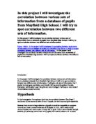
Key Stage 4 Girls’ Height
Table of Values of Histogram [Key Stage 4 Girl's Height]:
Class Int. Mid. Int. (x) Class Width Freq. Cum. Freq.
1.4 = x < 1.45 1.425 0.05 1 1
1.45 = x < 1.5 1.475 0.05 0 1
1.5 = x < 1.55 1.525 0.05 1 2
1.55 = x < 1.6 1.575 0.05 4 6
1.6 = x < 1.65 1.625 0.05 3 9
1.65 = x < 1.7 1.675 0.05 2 11
1.7 = x < 1.75 1.725 0.05 1 12
1.75 = x < 1.8 1.775 0.05 1 13
∑f = 13
∑fx = 20.97
∑fx² = 33.94
Mean = 1.613
Standard Deviation = 0.08583
Variance = 0.007367
Key Stage 4 Boys’ Height
Table of Values of Histogram [Key Stage 4 Boy's Height]:
Class Int. Mid. Int. (x) Class Width Freq. Cum. Freq.
1.5 = x < 1.55 1.525 0.05 1 1
1.55 = x < 1.6 1.575 0.05 0 1
1.6 = x < 1.65 1.625 0.05 1 2
1.65 = x < 1.7 1.675 0.05 2 4
1.7 = x < 1.75 1.725 0.05 1 5
1.75 = x < 1.8 1.775 0.05 5 10
1.8 = x < 1.85 1.825 0.05 2 12
1.85 = x < 1.9 1.875 0.05 1 13
1.9 = x < 1.95 1.925 0.05 1 14
∑f = 14
∑fx = 24.55
∑fx² = 43.19
Mean = 1.754
Standard Deviation = 0.09949
Variance = 0.009898
Key Stage 4 Boy’s Height
Height & Weight of all Boys
Height & Weight of all Girls
The scatter diagram above is for all girls in Mayfield high. It shows a strong positive correlation between the height and weight of all girls. The equation of the line of best fit is y= 20.54+ 37.5. The centroid of all my points lies on the co-ordinates (1.584,49.32). The positive correlation shows that the taller you are the heavier you are. The above strong correlation confirms my third hypothesis saying the taller you are the heavier you are.