I am going to find the mean, median and mode to help me prove that my hypothesis is correct
I will make sure that the survey is not biased, as I will choose the precautions mentioned above.
In the case of a word 2 letters long or less, I will choose the next word, because they will probably be outliers and will affect my results slightly. As shown in my pre-test, I did not use them. I did not use them because they are pronouns and are very common. If they were to be used they would affect the results greatly, and most of the small words have very few synonyms so cannot be changed.
Stratified Sampling
Tabloid
Total Pages – 28
There are 11 pages in the Tabloid devoted to News:
11 ÷ 28 × 100 = 40%.
40% of 150 = 60,
therefore I will take 60 words from News.
There are 9 pages of Sport in the Tabloid:
9 ÷ 28 × 100 = 32%.
32% of 150 = 48,
therefore I will take 48 words from Sport.
There are 8 pages of Finance in the Tabloid.
8 ÷ 28 × 100 = 28%.
28% of 150 = 42,
therefore I will take 42 words from Finance.
Broadsheet
Total Pages – 46
There are 24 pages in the Broadsheet which are in the News section:
24 ÷ 46 × 100 = 52%
52% of 150 = 78,
therefore I will take 78 words from News.
There are 8 pages of Sport in the Broadsheet:
8 ÷ 46 × 100 = 17%.
17% of 150 = 25.5,
I will round this up to 26, therefore I will take 26 words from Sport.
There are 14 pages in the Broadsheet devoted to Finance:
14 ÷ 46 × 100 = 31%
31% of 150 = 46.5,
I will round this down to 46, so I will take 46 pages from Finance
Full Results
Tabloid
Broadsheet
Analysis of Results
Tabloid
Mode: 4. This is the group with the highest frequency.
Mean: 821 ÷ 150 = 5.473˙.
Lower Quartile (Q1): 4. This is (150+1) ÷ 4 = 37.75 (38th value). This value is in the group of 4.
Median (Q2): 5. I worked this out by doing: ½(n+1) = ½(150+1) =
½ × 151 = 75.5 (76th value), which is in the group of 5.
Upper Quartile (Q3): 7: I worked this out by finding the (3n+1)/4th value, which was 451/4 which is 112.75 (113th value). This is in the group of 7 letters.
Inter-quartile Range: 3. This is Q3 – Q1, which is 7.25 – 4.46 = 2.79.
Outliers: 1.5 × 3= 4.5. 4 – 4.5 = -0.5 (This means short words are not outliers). 7 + 4.5 = 11.5. Any words over 11 letters long are outliers. However, the longest word I have recorded is 11 letters long so therefore I do not have any outliers.
Range: 8. This is the range between the longest word (11) and the shortest word (3).
Broadsheet
Mode: 6
Mean: 705 ÷ 150 = 4.7.
Lower Quartile (Q1): 5. I worked this out by finding the 38th value.
Median (Q2): 6. I worked this out by finding the 75th value.
Upper Quartile (Q3): 7. I worked out the upper quartile by finding the 113th value, which is in the group of 7 letters.
Inter-Quartile Range: This is 2, which is 7 – 5.
Outliers: 1.5 × 2 = 3. 5 - 2 = 3. There are words under 3 letters long so no small outliers. 7 + 2 = 9. There are 6 words longer than 9 letters, so these are outliers. They could affect the data greatly but outliers close to the range may not affect it as harshly.
Range: 8.
The Broadsheet had a higher mode than Tabloid, which shows that the most used size of word is bigger in the Broadsheet (6) than the Tabloid (4). This supports my hypothesis that Broadsheets have longer words.
However, the mean is higher in the Tabloid than the Broadsheet. This could be because of the fact that the mode of the Tabloid (4 letters) made up 37 of the 150 words, compared to the mode of the Broadsheet (6 letters (frequency of 30). The mean is higher in the Tabloid, so this does not support my hypothesis. The middle 50% is higher in the Broadsheet than the Tabloid, which shows that it is made more of longer words than shorter words, whereas the Tabloid is made mostly of words either 4 letters or 5 letters long.
The Tabloid has no outliers, as all words are between 1 and 11 letters long. However, the Broadsheet has 6 “outliers”, all 10 and 11 letters long. Although 10-letter-long words in the Tabloid are not outliers, words that are 10 letters long are outliers in the Broadsheet. This is because the Broadsheet’s middle 50% is smaller than the Tabloids, so when the formula is applied, the range for outliers is bigger.
As you can see on the frequency polygons, Tabloids mode was 4 while Broadsheets mode was 6. Tabloid’s polygon is mainly based around groups of 4 and 5, as they are the highest groups, and other groups have far lower frequencies. In the Broadsheet polygon, it is shown that the data is more spread-out, and also that it was based around the groups of 4, 5, 6 and 7 letters. The Broadsheet drops quickly after group 6, but then slows down when approaching 9 letters. The final 2 groups have the same frequency, similar to Tabloid’s polygon, but with a slightly higher frequency. They both have the same amount of 5-letter words, but Broadsheet’s polygon stays higher towards the end, which supports my hypothesis that Broadsheets have longer words. The frequency of longer words in the Broadsheet is higher than in a Tabloid.
The box plot shows that the middle 50% of the Tabloid is larger than that of the Broadsheet. The Tabloid box plot also has a positive skew, which indicates that there are more words which are small (3-4 letters) than long (7-11 letters). It shows this because if there were not a lot of small words, but a lot of long ones, there would be a bigger gap between Q1 and Q2, than Q2 and Q3, so therefore it would have a negative skew. However, in the Tabloid box plot, there is a bigger gap between Q2 (the median) and Q3, so therefore it has a positive skew.
In the Broadsheet box plot, the middle 50% is even both sides, indicating that there is roughly the same amount of small words as larger ones. However, the Broadsheet box plot is further up the scale of the x axis than the Tabloid, which shows that there are more long words (longer words would bring the box plot further up the scale), which is also shown in the frequency polygon. However, Q3 is the same for both Broadsheet and Tabloids, which shows that there were quite a lot of 7 letter words in the data.
Evaluation of Strategy
I used a pre-test to determine whether stratified sampling was the right method to use. It was the right method to use, and I decided to use stratified sampling as it was a way that I could find data that represented the whole population. I used various methods to try and make the way of collecting data fairer: This included splitting a hyphenated word in 2, disregarding names, but keeping words in quotations. The test could have been fairer if I had used 1 and 2 letter words in the data, as it would include words which are common to newspapers. Although they could affect the results, they are still part of the newspaper, and do not fall into one of the groups that I avoided (numbers, names etc.). I could have used different newspapers, or newspapers from different days. That way, the data would be more varied, and if I chose 2 newspapers from different days, different words would appear as there would not be 2 articles about the same thing. A wrong number or sum in the working out could greatly affect the results, so I had to be very careful when working out the sums. I used a tally chart to record the data, but a mistake when reading the tallies could cause a problem when counting it up and adding in the frequencies. With the data, I created box plots, frequency polygons and pie charts. I could also have produced cumulative frequency charts, but I found that a frequency polygon represented the data better.
Conclusion
The pie charts and box plots support my hypothesis; in the pie charts, the biggest sector in the Tabloid was 4, whereas in the Broadsheet the biggest was 6. In the box plots, it was shown that the lower quartile, median, and upper quartile were all higher in the Broadsheet than the Tabloid. There were more longer words in the Broadsheet, which is shown in the box plots where the median is much higher. However, the mean was higher in the Tabloid than the Broadsheet, which is against my hypothesis. The box plots and frequency polygons show that the Broadsheet is made of longer words than the Tabloid, however, the Broadsheet still has a lot of short words. In conclusion, my hypothesis was correct: There are longer words in a Broadsheet, so therefore they are harder to read. However, because of the means of both newspapers, the hypothesis could be unproven.
Second Hypothesis
Hypothesis: The percentage of text in a Broadsheet newspaper is higher than that of a Tabloid Newspaper.
I chose this hypothesis because in the previous hypothesis, which was correct, it was stated that Broadsheets had longer words. If they have longer words, they possibly take up more of the page. However, because of the size difference between Tabloids and Broadsheets, the area of the text would be bigger in the Broadsheet, as there is more area to fill in. I found the area of the paper that was made from text, so that I could compare both newspapers without any problems.
Plan
I will use percentage area, instead of normal area (cm2), because if I use length (cm), it would be biased towards the broadsheet, as they are much bigger than tabloids anyway. Therefore, the area would be higher in broadsheet. So, to make it fair, I will take the area of text in the page, divide it by the area of the whole page, and multiply the answer by 100. This will give me a percentage, which I will then put into a tally chart. I will then transform the completed tally charts into cumulative frequency tables. To choose the pages, I will use stratified sampling to find out how many pages I am going to take from each section – I will take 30 pages in total (from each paper). I will use this as it will show a fair representation of the data. From each section, I will choose the first x pages (x being the number of pages required). I will then create cumulative frequency graphs, histograms and box plots to help compare the two newspapers, in order to fine whether my hypothesis was correct or not. However, the data also relies upon the font and size of the text; if the Tabloid uses a bigger font than the Broadsheet, and also uses a slightly bigger text, the percentage area of text will be bigger in the Tabloid, due to unfair results.
Stratified Sampling
Tabloid
Total Pages – 28
there are 11 pages in the Tabloid devoted to News:
11 ÷ 28 × 100 = 40%.
40% of 30 = 12,
therefore I will take 12 pages from News.
There are 9 pages of Sport in the Tabloid:
9 ÷ 28 × 100 = 32%.
32% of 30 = 9.6. I will round this up to 10;
therefore I will take 10 pages from Sport.
There are 8 pages of Finance in the Tabloid.
8 ÷ 28 × 100 = 28%.
28% of 15 = 8.4.
I will round this down to 8; therefore I will take 8 pages from Finance.
Broadsheet
Total Pages – 46
there are 24 pages in the Broadsheet which are in the News section:
24 ÷ 46 × 100 = 52%
52% of 30 = 15.6,
I will round this up to 16; therefore I will take 16 pages from News.
There are 8 pages of Sport in the Broadsheet:
8 ÷ 46 × 100 = 17%.
17% of 30 = 5.1,
I will round this down to 5, therefore I will take 5 pages from Sport.
There are 14 pages in the Broadsheet devoted to Finance:
14 ÷ 46 × 100 = 31%
31% of 30 = 9.3,
I will round this down to 9, so I will take 9 pages from Sport.
Results
Tabloid
Broadsheet
I chose the groups because I believed that the frequencies would be more spread out if I had them that way. I also chose the groups so that the frequency densities kept similar at low figures. By using different class widths, I would be able to produce a more varied histogram. Although the class widths were different, I used multiples of five so that the histogram would be varied, but the frequency density would not be varied a lot.
Analysis of Results (Including Graphs)
Tabloid mean = ∑ (fx) ÷ ∑f = 1687.5 ÷ 30 = 56.25. An average page in a tabloid newspaper is made up of 56.25% text, and the rest pictures or adverts.
Broadsheet Mean = ∑ (fx) ÷ ∑f = 1812.5 ÷ 30 = 60.416˙, which I will round up to 60.42 to make the figures easier to handle. An average page in a broadsheet newspaper is made up of 60.42% text, and the rest pictures or adverts.
Tabloid
Mode: 50≤a<60
Lower Quartile (Q1): 35. I read this from the cumulative frequency graph.
Median (Q2): 56.5. I read this from the cumulative frequency graph.
Upper Quartile (Q3): 72.5: I read this from the cumulative frequency graph.
Inter-quartile Range: 37.5. This is Q3 – Q1, which is 72.5 – 35 = 37.5.
Broadsheet
Mode: 60≤a<75
Lower Quartile (Q1): 52. I read this from the cumulative frequency graph.
Median (Q2): 62.5. I read this from the cumulative frequency graph.
Upper Quartile (Q3): 72.5: I read this from the cumulative frequency graph.15, which is 12.5, and added it on to 60, to get 72.5.
Inter-quartile Range: 20.5. This is 72.5 – 52 (Q1-Q3) = 20.5.
The largest box on the Tabloid histogram is the group 50≤a<75, which represents the frequency of 9. This is the mode. The smallest box is 0≤a<20, which represents 1. This could be the smallest because newspapers are generally made of text, and sometimes have pictures in them. They are made to inform, but pictures do not inform as well as words. Tabloids like pictures, but still need to include text.
On the Broadsheet histogram, the biggest box by far is the box for 60≤a<75, which represents a frequency of 9. This is because Broadsheets are made up of more text (and longer words, as shown in first hypothesis), and so there is less room for pictures.
It is shown on the box plots that the Broadsheet’s quartiles are higher than the Tabloids. This shows that the Broadsheet uses more percentage area as text than the Tabloid does. The cumulative frequency curve shows that Broadsheet rises much later than Tabloid, showing that they later groups have higher frequencies (i.e. there is more percentage area text).
Evaluation of Strategy
First, I got my data using stratified sampling so that I could get a representation of the whole population when my results were finalized. However, a single wrong number could greatly affect the results, so I was careful when doing sums. I created histograms, frequency polygons, cumulative frequency curves and box plots to show the data, however, a wrong number could cause a major problem with the results. With the tally charts that I first used to record the data and frequencies, while adding them up, it is possible that I could have mis-read the tallies incorrectly, but this would not affect the results badly. Sometimes, wrong calculations could make the results support the hypothesis even more. ~
Conclusion
In conclusion, I found that my hypotheses were correct. Broadsheet had a higher median than Tabloid, and also had a higher mean. This means that Broadsheets must have a higher percentage area of text (in general) for the median and mean to be higher than Tabloid. Although a lot of factors such as text size, and also the font used (different fonts have different sizes and styles) come into practice regarding the overall area of the text, it is up to the newspaper editors to decide how much of the newspaper is text, how much is pictures, and how much advertising they show/offer. This data varies from paper to paper, and also the size of the business that runs the newspaper may affect the size of the layout: A small newspaper may need to give a lot of advertising space so that they can survive, and can only afford to print text, whereas a top-selling tabloid could offer a lot of pictures as they would have the money to print them in colour, and in black and white.
Overall Conclusion
In conclusion, I found that both my hypotheses were correct – and that they linked with each other. Newspapers (i.e. Broadsheets) with longer words would have to take up more area as text because otherwise their articles would be very short and possible would lose interest quickly. Tabloids, I have found, like to use shorter words, and they also use less text, as pictures, which they use a lot of, are likely to attract people in their target audience – young adults. Broadsheets however, with longer words and more text, may appeal to the older audience more.