*If neither person did the survey for any reason, then the gaps will be left blank.
The table above shows that I got most of my surveys back (43 of 52 to be precise). This means that my results probably will reflect what the whole of KS3 think, as every form (bar two) gave me at least one response to my survey.
I will show the results for each question in its relative hypothesis, and see whether their opinions were correct, and compare their opinions to what I thought.
Hypothesis one:
(On average, newspapers will have longer words in their articles than in magazines)
First of all, I am going to select four articles. Two of them will be from the newspapers (one from each), and the other two will be from two of my magazines (again, one from each). These are:
Article 1: ‘Health scare as girls of 7 diet to be like Geri’ (Daily Express, page 7)
Article 2: ‘Rivaldo too gifted to be remembered as a World Cup cheat’ (Daily Mirror, page 62)
Article 3: ‘Too fat too young’ (What’s on TV, page 83)
Article 4: ‘Big in Japan’ (Shoot monthly, from page 10)
Although this sounds straight forward, there are several things that could affect my results. For example, you may not be able to use certain words when comparing their lengths, because the editors have to put them in, not because they choose to. Because of this I have chosen not to include some parts of the article in my investigations. These are:
- Any speech – because the paper can’t control what people say, and so the editor can’t amend them to make the words in them longer or shorter
- Acronyms – because these are not words
- Names (of people, places and brand names) – again, the paper can’t control how long these names are
Also, there will be some other differences, such as:
- Numbers will be counted as words. For example, 12 will be counted as a six letter word, because it is written as TWELVE
- Hyphenated words will be counted as more than one word (unless it is there to show a word ends on the next line), because in most cases you would pronounce them as being more than one word. For example, north-west would be pronounced as “north west”
- Words with apostrophes in them will be counted as one word, because they are usually pronounced as one word. For example, world’s is pronounced as “worlds”
- Abbreviations will be counted as a word, but as its original state. For example, TV will be counted as a 10-letter word, because in its original state, it’s written as TELEVISION
From these articles, I am going to count how many letters there are in each of the first 100 words of the article, and then put my findings into the tally chart on the next page, which consists of a tally chart column, a total column (which is the total number of words with the corresponding number of letters in it), and the ∑f row at the bottom, which is the total frequency (which should always equal 100)
Mean length of words for newspapers (Articles one and two):
Mean = ∑fX ÷ ∑f
(Mean = The total of fX ÷ The total number of words)
Mean = 453 ÷ 100
Mean = 4.53 letters per word
Standard Deviation of the results:
S.D. = √ ( ∑f(X – X)² ÷ ∑f )
S.D. = √ 539.910005 ÷ 100
S.D. = √ 5.39910005
S.D. = 2.323596361
This means that 67% of all the results are within 2.32 (approx.) letters of the mean, which was 4.53.
Mean length of words for magazines (articles three and four):
Mean = ∑fX ÷ ∑f
(Mean = The total of fX ÷ The total number of words)
Mean = 448.5 ÷ 100
Mean = 4.485 letters per word
Standard Deviation of the results:
S.D. = √ ( ∑f(X – X)² ÷ ∑f )
S.D. = √ 565.9775 ÷ 100
S.D. = √ 5.659775
S.D. = 2.379028163
This means that 67% of all the results are within 2.37 (approx.) letters of the mean, which was 4.485
This shows that the standard deviations of both averages are very similar, as the differences between them is only 0.05 (2.37 – 2.32). This also reflects the small difference between the averages:
4.53 – 4.485 = 0.045 letters per word
As you can see, I proved my hypothesis was correct, although I was expecting a much larger difference between the two mean averages. On the next few pages there are several graphs to represent this data in many different ways, mainly to compare the two.
This also shows that the mean AND standard deviation between magazines and newspapers have a very close relationship with each other. This means that the results were almost identical.
Graph 1.1 (page 10):
This graph is a cumulative frequency graph. As you can see, the graph seems to be correct, because it is in the ‘S’ shape that all cumulative frequency graphs end up being in. The lines are in very similar positions, which reflect on the tiny difference between the averages of the difference in letters per word. The red line that represents magazines, shows there are slightly more words that are between 3-6 letters and 8-10 letters long. After these (7 and 11-12 letters), there are more letters per word, because the lines even out again.
Apart from this, the blue line (representing newspapers), and the red line are virtually identical, meaning there are the same numbers of letters per word up to that point on the graph.
Graph 1.2 (page 11):
This is a line graph representing each individual result, and not the cumulative frequency, and again, the blue line represents newspapers and the red line represents magazines. Unlike the cumulative frequency graph, these results are fairly different in most letter categories, but never the less follow the same trend.
The only two major exceptions to the trend are in the five-letter category - where in the newspapers there are more words than in the four-letter category; whereas in magazines there are fewer words than in the four-letter category - and in the seven-letter category - where in newspapers there are more words than in the six letter category; whereas in magazines there are less words in the six-letter category.
The green line represents the general trend of both graphs. It shows that the general trend is positively skewed, because the mean is greater than the median and the mode – which is telling us that as you go further along the ‘x’ axis, there is a less and less number being represented on the ‘y’ axis. This is why the mean is higher – because the mean is affected by smaller amounts of possible anomalous results, whereas the median and mode aren’t, and because the anomalous results appear to be the higher letter frequencies, then this will make the mean a greater number.
Survey results:
*Percentages to nearest whole number
This shows that the year seven’s had the best idea of what the answer turned out to be, because the answers they gave were the most similar in number (with a range of four), which reflects upon the similarity of the number of letters per word on average.
This also shows that the whole of KS3 would be correct, as the majority (74%) thought that newspapers would have the longer words on average.
Hypothesis two:
(There will be more articles in newspapers than in magazines)
For this, I am going to use a similar method to the one I used in hypothesis one, except I am going to use the first 40 pages from the magazines and newspapers, and I am going to use class intervals of five pages to make my results table easier to understand.
Here are the newspapers and magazines I will be using (details of them can be found on page one):
Newspaper 1: Daily Express Magazine 1: F1 Magazine
Newspaper 2: Daily Mirror Magazine 2: Shoot Monthly
From these, I will count the number of articles on each page, and input the data into the relevant box, as a tally at first, but then as overall totals later.
There are only two major problems I see with this. The first one is that if an article begins on one page in one interval and finishing on another page in a different interval. To solve this, I am simply going to say that any article will be classed to be on the page it begins on. For example, if there were a double page spread on pages 20 and 21, then it would go in the 16-20 category because the article starts on page 20.
The second problem is that if the magazines start on page 4 or 5, due to the contents or an introduction etc. at the beginning. To solve this, I am going to simply put a ‘0’ in the 1-5 if this occurs, because if I didn’t, it would make the graphs a lot harder to compare and the tables more confusing.
As you can see, it doesn’t take too much common sense to realise that hypothesis two is again correct. For the sake of preciseness though, I will work out the mean averages:
Mean average for newspapers:
X = ∑X ÷ N
(Mean = The total of the single frequencies ÷ the number of frequencies)
Mean = 52.5 ÷ 8
Mean = 6.56 articles per interval, which means… 6.56 ÷ 5 = 1.31 articles per page
Mean average for magazines:
X = ∑X ÷ N
(Mean = The total of the single frequencies ÷ the number of frequencies
Mean = 18.5 ÷ 8
Mean = 2.31 articles per interval, which means… 2.31 ÷ 5 = 0.46 articles per page
The difference between the no. of articles per page: 1.31 – 0.46 = 0.85
Although this looks as if it was pretty fair, I think that part of the problem with the magazines is that some articles were several pages long, and there were a lot more pictures in them. Never the less, the point of the hypothesis was to find the number of articles despite these kind of problems, so this hypothesis must be correct.
Graph 2.1 (page 16):
This is a graph to show the correlation between the two variables. Unlike in the graphs on pages 6 and 7, these points aren’t joined up together. This is because we are looking to see how well the lines would fit together supposing we put them on a line of best fit. You can see a blue line on this as well – this is a regression line, which is simply a line of best fit.
There is a point on the graph at (6.56, 2.31) that this line goes through, this is the co-ordinate that shows the average frequencies for both the ‘x’ and ‘y’ axis (i.e. 6.36 and 2.31 are the average frequencies of articles in newspapers and magazines per page). The working out for this is on page 15. This has given me some idea of where to place my line of best fit to make it correct. I don’t think it shows the line of best fit too well, but only because the circled anomalous result made the average co-ordinates larger than they would have been supposing it wasn’t there.
Coefficient of rank correlation for newspapers and magazine (for basic details on correlation, see page 1):
R = 1 - __6∑d²__
n(n² - 1)
R = 1 - __6 x 71__ = 1 – (426 ÷ 504) = 1 – 0.84 = 0.16
8(64 – 1)
This shows that the correlation between the number of magazine and newspaper articles per page is very low. This is what I was expecting to happen on the graph, as the results seemed to be scattered in no particular order. Especially with taking the anomalous result (circled on graph) into account, the results of this formula seem to have come out right.
Regression line equation:
Average frequency for newspapers (x axis):
X = ∑X ÷ N
Mean = 52.5 ÷ 8 = 6.56
Average frequencies for magazines (y axis):
X = ∑X ÷ N
Mean = 18.5 ÷ 8 = 2.31
Average co-ordinates (x, y): (6.56, 2.31)
Survey results:
*Percentages to nearest whole number
Although I was correct, KS3 seemed to think that the answer overwhelmingly was magazines, which in fact means that the majority of people were wrong. This also means that no individual year was right, either. However, year 8 was technically the most correct, because the highest percentage of answers saying it was newspapers came from year 8.
Hypothesis three:
(Magazine supplements from newspapers will have longer words than ordinary magazines)
For this, I’m going to use the same method that I used in hypothesis one. This time though, I am going to use only two articles, because I’ve got two appropriate magazines that are as similar as you can get – so I don’t see the need to use more. This is because they are both of the same type, and they are from the same dates they are to be used for – they even had the same photo in them! This means that there should be absolutely nothing that can affect the outcome of my results.
The two magazines and articles I use will be (details of the magazines can be found on page 1):
Magazine supplement: The TV mag - Shipman (page 82)
Magazine: What’s on TV - Shipman (page 15)
Mean length of words for magazine supplements and magazines:
* ∑f = 100
Magazine supplements:
Mean = ∑fX ÷ ∑f
Mean = 454 ÷ 100 = 4.54 letters per word
Magazines:
Mean = ∑fX ÷ ∑f
Mean = 495 ÷ 100 = 4.95 letters per word
Difference: 4.95 – 4.54 = 0.41 letters per word
This shows that magazines have more letters per word in them, so my hypothesis in this case was wrong. I think this may be because the magazine supplement writers may want to write as if it is a magazine and not a newspaper – and in this case it happened to have less letters per word. I therefore think that no matter how many articles you tested, I think that you would get pretty similar results all the time (as we did here with a difference of only 0.41 letters per word).
Graph 3.1 (page 20):
This is another cumulative frequency graph, but this time I have got some points marked on representing the interquartile ranges for the data. The lines that come from 25, 50 and 75 on the ‘y’ axis are Q1 (0.25 x ∑f), Q2 (0.5 x ∑f) and Q3 (0.75 x ∑f) respectively. Q2 is also the median. (details of this can be found on page two).
The interquartile range is a different kind of average used so that we can see how the data is scattered around the averages, (in other words, it accounts for anomalous results unlike the mean, as well as the range of the figures).
Q3 – Q1 = 0.75(∑f) – 0.25(∑f)
Interquartile range for magazine supplements: Interquartile range for magazines:
(to the nearest 0.1) (to the nearest 0.1)
Q1 = 2.3 Q2 = 3.4 Q3 = 5.3 Q1 = 2.5 Q2 = 3.7 Q3 = 5.9
5.3 – 2.3 = 3 letters per word 5.9 – 2.5 = 3.4 letters per word
3.4 – 3 = 0.4 letters per word difference
This shows that although the actual numbers in the interquartile range don’t seem to be that accurate compared to the mean average, the difference between the magazine and the supplement is almost identical to that of when I found it out using the ‘mean = ∑fX ÷ ∑f’ method.
Graph 3.2 (page 21):
This is a composite bar chart to show the numbers of words with each letter found in the magazine and supplement – but when they are put together in the same graph. The ‘x’ axis is the axis with the no. of letters on it. It has the numbers 1-14 on, so that the numbers of words with the corresponding no. of letters can be put on. The ‘y’ axis is the no. of words axis. This goes up to 60 to accommodate for the 28 + 23 total from the 3-letter word category.
You can see that the magazine supplement scale is in blue, and straight above them there are the magazine scales in red. This is so that neither one gets confused with the other. I think although it can’t tell you the exact amounts of words for the magazines, I think it’s a very good way to compare the two.
The green line represents the general trend of both frequencies together. It shows that it is positively skewed, because the mean is greater than the median and the mode – which is telling us that as you go further along the ‘x’ axis, there is a less and less number being represented on the ‘y’ axis. This is why the mean is higher – because the mean is affected by smaller amounts of possible anomalous results, whereas the median and mode aren’t, and because the anomalous results appear to be the higher letter frequencies, then this will make the mean a greater number, and not smaller.
Survey results:
*Percentages to nearest whole number
This shows that each individual year, and KS3 as a whole, were much more unsure of what the answer was this time. This is shown by the similarities between the percentages of each. Year 9's were the most accurate with their answers, as the highest percentage of answers (54%) went to magazines.
However, the majority of KS3 (49%) thought that the answer was the magazine supplements, so like me, they were wrong.
Hypothesis four:
(There will be more adverts in magazines)
For this hypothesis, I am going to use the same method that I used in hypothesis two (counting the frequencies of the adverts on the first 40 pages). The only exception is that I am going to count all the different types of advert that are in the newspapers and adverts, e.g. for electrical appliances or food.
Newspapers and magazines that I will be using (details of them can be found on page one):
Newspaper one: Daily Mirror Magazine one: F1 Racing
Newspaper two: Daily Express Magazine two: Shoot Monthly
Although this sounds straight forward, I think I will have the problem of having some adverts coming under two separate categories. In this case, I will assign it to the type it is more compatible for. For example, if I saw an advert that advertises a department store, then I will assign it to the type of item it is selling it.
Here are the types of adverts I will be using:
- Electrical or electrical appliances
- Services (e.g. compensation ads, plumbing)
- Food and drink (e.g. supermarkets)
- Travel (e.g. travel agents or cars)
- Clothing and things you wear on your body (e.g. glasses)
- Furniture
- Ordinary non-food products
- DIY/garden
- Other
This clearly shows that there are far more adverts in newspapers, and so this proves my hypothesis wrong. I also noticed that in the magazines, there were a lot of adverts suited towards its topic. For example, in ‘F1 Racing’ (magazine 1), there are a lot of adverts under travel, and in ‘Shoot Monthly’, there was a lot under clothes/things you wear (especially with brand names such as Adidas).
No of adverts in newspapers: (24 + 35) ÷ 2 = 29.5 ads per 40 pages.
29.5 ÷ 40 = 0.74 ads per page.
No. of adverts in magazines: (6 + 9) ÷ 2 = 7.5 ads per 40 pages.
7.5 ÷ 40 = 0.19 ads per page.
Difference: 0.74 – 0.19 = 0.55 ads per page.
I will back these results up by finding the average frequency…
Average frequency of adverts in newspapers:
This time, the frequency (f) becomes X. This is because the type of advert column doesn’t need to be tampered with, unlike it needed to be in the other calculations. Also, N becomes 40 (the no. of pages involved with the hypothesis investigation), because we are looking for the number of adverts per page, and not per category. This is simply for purposes so we can compare them within the table.
*The last column may not be accurate, because all the numbers added together must equal 360°
Average frequency for adverts in magazines:
*The last column may not be accurate, because all the numbers added together must equal 360°
**All the types with a dash in them wont be included, unlike for in the newspapers
Average frequency for number of adverts in newspapers:
X = ∑X ÷ N
Mean = 29.5 ÷ 40 = 0.74 adverts per page
Average frequency for number of adverts in magazines:
X = ∑X ÷ N
Mean = 7.5 ÷ 40 = 0.19 adverts per page
Graph 4.1 (page 26):
These are pie charts to show the number of adverts in newspapers and magazines corresponding to their subject, according to the results in the tables on page 22.
Graph 4.2 (page 27):
This is a composite histogram with a frequency polygon. In the two tables on page 18, I actually set the advert type column up in a specific way. I put the type of item I thought would be most common up at the top, and the item I thought I would see the less at the bottom (along with ‘other’). So, the purpose of this frequency polygon is to see whether I was correct. It will signal I am correct if the polygon gradually descends as it moves from left to right on the graph.
The results of the graph show that I was partially correct, although I made a few mistakes (like greatly underestimating the number of services), which mean I was partially wrong, too.
Survey results:
*Percentages to nearest whole number
This shows that, unlike me, the whole of KS3, and each individual year, were in fact correct, thinking that newspapers had more adverts in them. Not only this, but overall, the majority was quite overwhelming (with 60%).
The most accurate year 7, because they were the year which had the highest percentage of the surveyed people thinking the answer was newspapers.
This means that the year, which have tended to be correct the most is in fact year 7, by being the most accurate for two of the hypotheses. Years 8 and nine were both the most accurate in one hypothesis.
Conclusion:
Overall, I got two hypotheses correct and two hypotheses incorrect. This shows I could predict some differences between newspapers and magazines, but not all of them. This also shows that doing this investigation was a good thing, because if I didn’t, I would have carried on thinking that these incorrect hypotheses were correct.
This also showed me that KS3 could predict what the answer to my hypotheses are, as they got the answers to three of my four questions, with each question based on one hypothesis, correct.
However, there were limitations to how accurate I can say my results actually are. There are several reasons for this. These reasons are:
- I only asked people within Kirk Balk School for their opinions. This means that I haven't covered opinions of people with different ages, different professions (and to a lesser extent with different wages/salaries), and from different areas other than party of the Barnsley region, who could all show different opinions.
- In hypothesis one, I described all the ways I will use the words in the article (e.g. count numbers as what they would say in word form), and how I wouldn’t count some words as words, whether or not they couldn’t be controlled by the newspaper or magazine. Perhaps I should have counted speech, as people speaking to different genre of the paparazzi would adjust their vocabulary use depending on whom they were speaking to. For example, perhaps people talking to broadsheet newspapers would tend to use larger words than people who talk to tabloid newspapers.
- Leading on from this, perhaps I should have found the average results of the number of words from tabloid newspapers and broadsheet newspapers, and then compared them with magazines. I wasn’t too careful about this, as I thought that any newspaper is a newspaper at the end of the day, but later, I began to wonder if I should have done this. This is because, I presume that broadsheet newspapers tend to use larger words than tabloid newspapers; to suit the more ‘educated’ reader, as I said in the previous point. However, I did inadvertently use a newspaper, The Daily Express, which can’t be classed as a broadsheet, as it has A4 pages, but did seem to be aimed at a more ‘educated’ audience, which does make up for the lack of broadsheet papers in a way.
- In hypotheses two and four, I used intervals of 4 pages, which perhaps were too small overall. This is because some articles and adverts, particularly in magazines, tended to begin in one interval and end in another. At least with larger intervals, this would happen less (as a percentage of all articles), and therefore make my results more reliable.
- Perhaps with hypothesis one, I should have tried to use as similar articles as possible. This is because then there wouldn’t be any differences between what was being written. For example, in hypothesis three, I picked two articles that were describing the same thing, the television show ‘Shipman’, which at the times was about to be shown on television. Because they are describing the same thing, there can be no differences between the words used, other than the writers and/or editors choice of vocabulary.
Despite these problems, I am satisfied that the results I got from the data were accurate, even to say that some results didn’t match what I thought the results should have been prior to doing the tests.