I drew the graphs from the data given. It includes 100 cars and their information.
Summarise and Interpret Data:
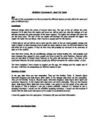
This graph shows that the older a car is the lower in price it becomes. It also shows moderate negative correlation. The equation of this graph is y=-0.0008x+8.832. This is appropriate because it shows that for every year that the car gets older it loses £900 in value. It can be used to predict the price of a second hand car depending on the age. The mean of the data is 5.33 years. The median is 6 years.
The lower quartile is 3 years and the upper quartile is 7 years. This is shown in the box plot. The Inter Quartile Range is the distance between the lower and upper quartiles in this set of data it is 4.
There are 11 outliers in this data. They are found by using the equations :
LQ - 1.5 x IQR and UQ + 1.5 x IQR.
In this case the equations are as follows:
3-1.5x4=-3
7+1.5x4=13
The outliers therefore are below 3 years and above 13 years
Outliers
I will remove these outliers to make my data more accurate.
This is a grouped frequency table of the age data. This will be used to draw a cumulative frequency graph.
Summarise and Interpret Data
This graph shows that the higher the mileage the lower the price of a car. It shows moderate negative correlation. The equation of the graph is y=-0.0775x+7876.1. It is appropriate and it can be used to predict the price of the car depending on the mileage. The mean of the data is 43,753 miles. The median is 43,000 miles. The lower quartile is 27,000 miles and the upper quartile of the data is 55,000 miles. These were found using Excel. The inter quartile range for this data is 28,000 miles.
In this data there are 12 outliers. Theses are found by using the equations:
LQ - 1.5 x IQR and
UQ + 1.5 x IQR
In this case it means that the outliers are less than 15,000 miles and over 97,000 miles.
Outliers
These outliers will be removed to make the data more accurate.
A grouped frequency table has been drawn to sort the data. It will then be used to draw a cumulative frequency graph.
Summarise and Interpret Data:
This graph has positive correlation. This shows the larger the engine size the more expensive the car is. The equation of the graph is y=3749.5x-1253. This is appropriate and can be used to predict the second hand price of a car depending on the engine size. The mean of the data is 1.6, the median is 1.6, the lower quartile is 1.3 and the upper quartile is 1.8. The inter quartile range of the data is 0.5.
The outliers in this data are underneath 0.55 and over 2.55.
1.3-1.5 x 0.5=0.55
1.8+1.5x0.5=2.55
Outliers
These values have already been removed because they were anomalies.
A grouped frequency table will now be drawn to sort the data information. This will then be turned into a frequency graph.
Summarise and Interpret Data
Now I decided to look at the prices of Ford, Rover and Vauxhall cars. I found out who keeps the price better and which make of car loses the most value. Then I worked out the mean percentage drop in price. I did this by using different functions on Excel Spreadsheet. Firstly I had to find how much the price dropped then I divided the drop by the original price to find the percentage. Then I found the mean percentage for the three makes of car. They are as follows:
Rover: 73.45(2d.p)%
Ford: 66.42(2d.p)%
Vauxhall: 61.19(2d.p)%
This means that out of these three makes of car Vauxhall keeps its second hand value better than Ford or Rover. I also found out if the number of previous owners affected the price of the car. These are my results:
1 previous owner: drop of 53.43%(2d.p)
2 previous owners: drop of 65.72% (2d.p)
3 previous owners: drop of 79.69% (2d.p)
This shows that the amount of previous owners does affect the price decrease. The more owners the car has had the more it drops in value.
Conclusion:
The work I have done shows that different factors affect the price decrease. For example the mileage affects the price. For every mile that the car drives it decreases in price. Also the number of owners, the age and the engine size all affect the price.
It also shows that my hypothesis is true. The more a second hand car is used the more it decreases in price. Also, extras mean that the car will be slightly more expensive. This is because they are not necessities in the car but luxuries, so more is paid because they need to be fitted. A car decreases in price if it has more mileage, owners or is higher in age because it has been used more. This means that the newer a car is, for example a car that is one year old, has had one owner and has a low mileage, will drop less in price because it is almost new.
To improve my coursework I could gather more data to make everything more accurate and give me a better example of how prices in second hand cars decrease. Also I could do extra comparisons and more analysis of different variables.
I also decided to see if the number of owners that a car has had will affect the price.
1 previous owner: drop of 53.43%(2d.p)
2 previous owners: drop of 65.72% (2d.p)
3 previous owners: drop of 79.69% (2d.p)
4 previous owners: drop of 82.14% (2d.p
This graph shows that the amount of previous owners does affect the price decrease. The more owners the car has had the more the price drops. At first the price decreases by around 12% or 13% but then it begins to slow down and the decrease from 3 owners to 4 owners is only 2.45%. I predict that if I collected extra data and found cars that had more owners then the price decrease would still rise but at a slower rate.