Graph: Y = -0.5x2
The table below shows the points, which I have used to plot the graph:
Gradients:
L1: Gradient at point X =-2
Y2-Y1
X2-X1
= -1-(-2.45) = 1.93 rounded to 2 d.p
-1.5-(-2.25)
L2: Gradient at point X=1
Y2-Y1
X2-X1
= -0.75-0 = -1.07 rounded to 2 d.p
1.25-0.55
L3: Gradient at X = 2
Y2-Y1
X2-X1
= -2.4-(-1.5) = -1.8
2.25-1.75
Graph: Y = -2x2
The table shows the points, which I have used to plot the graph:
Gradients:
L1: Gradient at point X = 1
Y2-Y1
X2-X1
= -1-(-2.5) = -5
0.85-1.15
L2: Gradient at X =0
Y2-Y1
X2-X1
= 0-0 = 0
0.5-(-0.5)
L3: Gradient at point X =-1
Y2-Y1
X2-X1
= -3-(-1) = 5
-1.2-(-0.8)
Graph: Y = x2
The table below shows the points, which I used to plot the graph:
Gradients:
L1: Gradient at point X = -1
Y2-Y1
X2-X1
= 2-0.5 = -2
-1.5-(-0.75)
L2: Gradient at point X = 1
Y2-Y1
X2-X1
= 2-0 = 2
1.5-0.5
L3: Gradient at point X = -2
= 5-4 = -4
-2.25-(-2)
Graph: Y = -0.5x3
The table below lists the points I have used to plot the graph:
Gradients:
L1: Gradient at point X = -2
Y2-Y1
X2-X1
= 5-3 = -5.71 rounded to 2 d.p
-2.2-(-1.85)
L2: Gradient at point X = 1
Y2-Y1
X2-X1
= -0.2-(-0.9) = -1.75
0.85-1.25
L3: Gradient at point X = 2
Y2-Y1
X2-X1
= -3-(-5) = -5
1.8-2.2
Graph: Y = -2x3
The table below shows the co-ordinates I have used to plot the graph:
Gradients:
L1: Gradient at point X = -2
Y2-Y1
X2-X1
= 20-12.5 = -25
-2.2-(-1.9)
L2: Gradient at point X = -1
Y2-Y1
X2-X1
= 5-0 = - 5.2
-1.56-(-0.6)
L3: Gradient at point X= 1
Y2-Y1
X2-X1
= -4.5-0 = -5.29 rounded to 2.d.p
1.5-0.65
Graph: Y= x3
The table below shows the points, which I have used to plot the graph:
Gradients:
L1: Gradient at point X = 2
Y2-Y1
X2-X1
= 12-3.5 = 11.33 rounded to 2.d.p
2.35-1.6
Gradient at point X = -2
Y2-Y1
X2-X1
= -2.5-(-11) = 11.33 rounded to 2.d.p
-1.5-(-2.25)
Gradient at point X = -3
Y2-Y1
X2-X1
= -17-(-29.5) = 25
-2.6-(-3.1)
I have now found the gradients of the different graphs, which I had planned to investigate using the tangent method. I will now check the accuracy of these results using the increment method.
Increment Method
I will now perform the small increment method to check my gradients. I will perform the increment method for each of the curved graphs i.e. the quadratic curves, the cubic curves and the hyperbolas. I will take 4 increments for all the tangents, which I have drawn. I will show the first calculation as an example for how I obtained the values in the table. From the table, I will take the gradient value, which is closest to my tangent value. I will take the increment gradient value, which is closest to my gradient from the tangent method. The increment method is very much like ‘zooming’ in on a point.
Graph: Y = 1/x
The table below shows the results from the increment method, where the tangent is at the point (1,1)
(X1, Y1) = 1,1
(X2, Y2) = 1.001, (1/X2)
(X2, Y2) = (1. 001, 0.999001)
Gradient = Y2-Y1/X2-X1
= 0.999001-1/1.001-1
= -0.999001
The table below shows the increment method performed, at the point (-2, -0.5)
(X1, Y1) = -2, -0.5
(X2, Y2) = -1.999, (1/X2)
(X2, Y2) = (-1.999, -0.50025)
Gradient = Y2-Y1/X2-X1
= -0.50025-(-0.5)/-1.999-(-2)
= -0.25013
The table below shows the increment method performed at the point (-1, -1)
(X1, Y1) = -1, -1
(X2, Y2) = -0.999, (1/X2)
(X2, Y2) = (-0.999, -1.001)
Gradient = Y2-Y1/X2-X1
= -1.001-(-1)/-0.999-(-1)
= -1.001
Graph: Y = 3/x
The table below shows the increment method performed at the point (2, 1.5)
(X1, Y1) = 2, 1.5
(X2, Y2) = 2.001, (3/X2)
(X2, Y2) = (2.001, 1.49925)
Gradient = Y2-Y1/X2-X1
= -1.49925-1.5/2.001-2
= -0.74963
The table below shows the increment method performed at the point (-2, -1.5)
(X1, Y1) = -2, -1.5
(X2, Y2) = -1.999, (3/X2)
(X2, Y2) = (-1.999, -1.50075)
Gradient = Y2-Y1/X2-X1
= -1.50075-(-1.5)/-1.999-(-2)
= -0.75037519
The table below shows the increment method performed at the point (-3, -1)
(X1, Y1) = -3, -1
(X2, Y2) = -2.999, (3/X2)
(X2, Y2) = (-2.999, -1.00033)
Gradient = Y2-Y1/X2-X1
= -1.00033-(-1)/-2.999-(-3)
= -0.33344448
Graph: Y = -2/x
The table below shows the increment method performed, at the point (-2, 1)
(X1, Y1) = -2, -1
(X2, Y2) = -1.999, (-2/X2)
(X2, Y2) = (-1.999, 1.0005)
Gradient = Y2-Y1/X2-X1
= 1.0005-1/-1.999-(-2)
= 0.50025013
The table below shows the increment method performed at the point (-3.5, 0.57)
(X1, Y1) = -3.5, 0.57
(X2, Y2) = -3.4, (-2/X2)
(X2, Y2) = (-3.4, 0.588)
Gradient = Y2-Y1/X2-X1
= 0.588-0.57/-3.4-(-3.5)
= 0.18
The table below shows the increment method performed at the point (2, -1)
(X1, Y1) = 2, -1
(X2, Y2) = 2.001, (-2/X2)
(X2, Y2) = (2.001, -0.9995)
Gradient = Y2-Y1/X2-X1
= -0.9995-(-1)/2.001-2
= 0.49975012
Comparison Between Tangent & Increment Method:
The table below shows the comparison between the values of gradient obtained from the tangent method and the increment method. Note: the values of the increment method have been rounded to 2.d.p
From the table above we can see that the increment method is much more accurate than the tangent method. Thus I will use the results from the increment method to the generalization of the gradient.
Generalization: Gradient Function For Graphs Of Y = a/x
To make the generalization easier I have drawn a table summarising the gradient found by the increment method at a common point in all the graphs.
From the table above we can see that gradient function for the hyperbolas is ‘-a x (1/x) 2
I will now test this equation on the above given points
X = -2 [Y = 1/x]
-a (1/x) 2
= -1(1/-2) 2
= -0.25
X = -2 [Y = -2/x]
-a (1/x) 2
= -(2)(1/-2) 2
= 0.5
X = -2 [Y = 3/x]
-a(1/x)2
= -(3)(1/-2) 2
= -0.75
From the above calculations I conclude that the gradient function of any hyperbola at point ‘x’ is obtained by:
-a (1/x) 2
Graph: Y =X2
The table below shows the increment method performed at the point (1,1).
The values of the gradient have been rounded to 2.d.p
(X1, Y1) = 1,1
(X2, Y2) = 1.001, (X2) 2
(X2, Y2) = (1.001, 1.002001)
Gradient = Y2-Y1/X2-X1
= 1.002001-1/1.001-1
= 2.00
We can see from the table above that the gradient at the point (1,1) is 2.
The table below shows the increment method performed at the point (-1,1)
(X1, Y1) = -1,1
(X2, Y2) = -0.999, (X2) 2
(X2, Y2) = (-0.999, 0.998001)
Gradient = Y2-Y1/X2-X1
= 0.998001-(-1)/ -0.999-1
= -2.00
From the table above we can see that the value of the gradient at the point X =-1 is 2, since all the increments when rounded to a whole number would give us the same value.
The table below shows the increment method performed at the point (-2,4)
(X1, Y1) = -2,4
(X2, Y2) = -1.999, (X2) 2
(X2, Y2) = (-1.999, 3.996001)
Gradient = Y2-Y1/X2-X1
= 3.996001-(-2)/ -1.999-4
= -4.00
From the table above we can easily see that the gradient at the point X = -2 is –4.
Graph: Y = -2x2
The table below shows the increment method performed at the point (-1, -2)
(X1, Y1) = -1, -2
(X2, Y2) = -0.999, -2(X2) 2
(X2, Y2) = (-0.999, -1.996)
Gradient = Y2-Y1/X2-X1
= -1.996-(-2)/ -0.999-(-1)
= 4.00
We can easily see, from the above increment method that the gradient, at the point (-1,2) is 4. There is a slight decrease in the gradient as you go down the X2 values, but this happens only because of the increasing increment. If the values are rounded off to whole numbers, the answer would still be the same, unless of course a very large increment is chosen.
The table below shows the increment method performed at the point (1, -2).
(X1, Y1) = 1, -2
(X2, Y2) = 1.001, -2(X2) 2
(X2, Y2) = (1.001, -2.004)
Gradient = Y2-Y1/X2-X1
= -2.004-(-2)/ 1.001-1
= -4.00
From the table above we can see that the gradient at the point (1, -2) is –4.
The table below shows the increment method performed at the point (0,0)
(X1, Y1) = 0, 0
(X2, Y2) = 0.001, -2(X2) 2
(X2, Y2) = (0.001, -0.0000002)
Gradient = Y2-Y1/X2-X1
= -0.0000002-0/ 0.001-0
= 0.00
From the table we see that the gradient at the point (0,0) is 0, however the gradient goes into negative values as the X2 values are increased.
Graph: Y =-0.5x2
The table below shows the increment method performed at the point (-2, -2)
(X1, Y1) = -2, -2
(X2, Y2) = -1.999, -0.5(X2) 2
(X2, Y2) = (-1.999, -1.998001)
Gradient = Y2-Y1/X2-X1
= -1.998001-(-2)/ -1.999-(-2)
= 2.00
From the table above we can clearly see that at the point (-2, -2) the gradient is 2.
The table below shows the increment method performed at the point (1, -0.5)
(X1, Y1) = 1, -0.5
(X2, Y2) = 1.001, -0.5(X2) 2
(X2, Y2) = (1.001, -0.501001)
Gradient = Y2-Y1/X2-X1
= -0.501001-(-0.5)/ 1.001-1
= -1.00
From the table above we can see that at the point (1, -0.5) the gradient is –1.
The table below shows the increment method performed at the point (2, -2)
(X1, Y1) = 2, -2
(X2, Y2) = 2.001, -0.5(X2) 2
(X2, Y2) = (2.001, -2.002001)
Gradient = Y2-Y1/X2-X1
= -2.002001-(-2)/ 2.001-2
= -2
From the table above we can see that the gradient at the point (2, -2) is –2.
Now I have performed the increment method for all the quadratic curves. I will now compare the gradients obtained by the tangent method with the gradients obtained by the increment method.
Comparison Between Tangent & Increment Method:
The table below shows the comparison between the values of the gradients obtained from the tangent method and the increment method:
From the table above we can see that increment method gradients are much more accurate than the tangent method, since in the tangent method a graph is required. The tangent can be drawn wrong if done manually, so I will take the increment method readings to find out the gradient function of the graphs Y =ax2
Generalization: Gradient Function For Graphs Of Y =ax2
To make the Generalization easier I have shown the gradient values from all the graphs at one common point. In this case at the point where X = 1
From the above table we can see that the gradient function of the graphs of Y=ax2 is:
2ax
I will now check my gradients for the above table using the above-calculated gradient function.
Gradient at point X = 2 [Y= x2]
= 2ax
= 2 x 1 x -2
= -4
Gradient at point X = 1 [Y= -2x2]
= 2ax
= 2 x -2 x 1
= -4
Gradient at point X = 1 [Y= -0.5x2]
= 2ax
= 2 x –0.5 x 1
= -1
My calculations show the gradient function to be accurate. I will now perform the increment method for the Graphs of Y = ax3 and then find the gradient function for them.
Graph: Y = X3
The table below shows the increment method performed at the point (2,8)
(X1, Y1) = 2, 8
(X2, Y2) = 2.001, (X2) 3
(X2, Y2) = (2.001, 8.012006)
Gradient = Y2-Y1/X2-X1
= 8.012006-8/ 2.001-2
= 12
The table above clearly shows that the gradient at the point (2,8) is 12.
The table below shows the increment method performed at the point (-2, -8)
(X1, Y1) = -2, -8
(X2, Y2) = -1.999, (X2) 3
(X2, Y2) = (-1.999, -7.988006)
Gradient = Y2-Y1/X2-X1
= -7.988006-(-8)/ -1.999-(-2)
= 12 [rounded to 1.d.p]
From the table above we can see that the gradient at the point (-2, -8) is 12, when rounded off to the nearest whole number.
The table below shows the increment method performed at the point (-3, -27)
(X1, Y1) = -3, -27
(X2, Y2) = -2.999, (X2) 3
(X2, Y2) = (-2.999, -26.97301)
Gradient = Y2-Y1/X2-X1
= -26.97301-(-27)/-2.999-(-3)
= 27 [rounded to 1.d.p]
From the table above we can see that the gradient at the point (-3, -27) is 27 when rounded off to the nearest whole number. The slightly less value of the gradient is because the increment method is not 100% accurate although it is 98-99% accurate.
Graph Y =-2x3
The table below shows the increment method performed at the point (1, -2)
(X1, Y1) = 1, -2
(X2, Y2) = 1.001, -2(X2) 3
(X2, Y2) = (1.001, -2.006006)
Gradient = Y2-Y1/X2-X1
= -2.006006-(-2)/ 1.001-1
= -6
From the table above we can see that the gradient at the point (1, -2) is –6.
The table below shows the increment method performed at the point (-1,2)
(X1, Y1) = -1, 2
(X2, Y2) = -0.999, -2(X2) 3
(X2, Y2) = (-0.999, 1.994006)
Gradient = Y2-Y1/X2-X1
= 1.994006-2/ -0.999-(-1)
= -6 [rounded to 1.d.p]
From the table above we can clearly see that the value of the gradient at the point (-1,2) is –6.
The table below shows the increment method performed at the point (-2, 16)
(X1, Y1) = -2, -16
(X2, Y2) = -1.999, -2(X2) 3
(X2, Y2) = (-0.999, 15.97601)
Gradient = Y2-Y1/X2-X1
= 15.97601-16/ -1.999-(-2)
= -24 [rounded to 1.d.p]
From the table above we can see that the gradient at the point (-2, 16) is –24 when rounded off to 1.d.p.
Graph: Y =-0.5x3
The table below shows the increment method performed at the point (1, -0.5)
(X1, Y1) = 1, -0.5
(X2, Y2) = 1.001, -0.5(X2) 3
(X2, Y2) = (1.001, -0.501502)
Gradient = Y2-Y1/X2-X1
= -0.501502-(-0.5)/ 1.001-1
= -1.5
From the table above we can clearly see that the gradient the point (1, -0.5) is –1.5.
The table below shows the increment method performed at the point (2, -4)
(X1, Y1) = 2, -4
(X2, Y2) = 2.001, -0.5(X2) 3
(X2, Y2) = (2.001, -4.006003)
Gradient = Y2-Y1/X2-X1
= -4.006003-(-4)/ 2.001-2
= -6
The table above clearly shows that the gradient at the point (2, -4) is –6.
The table below shows the increment method performed at the point (-2, 4)
(X1, Y1) = -2, 4
(X2, Y2) = -1.999, -0.5(X2) 3
(X2, Y2) = (-1.999, 3.994003)
Gradient = Y2-Y1/X2-X1
= 3.994003-4/ -1.999-(-2)
= -6 [rounded to 1.d.p]
From the table above we can see clearly that the gradient at the point (-2, 4) is –6.
I have now performed the increment method on all the cubic graphs. I will now compare the results of the gradients from the increment method with the gradients obtained from the tangent method.
Comparison Between Tangent & Increment Method:
The table below shows the comparison of the gradients obtained from the tangent method and the increment method:
From the table we again see that the tangent method is quite inaccurate, due to the inconsistencies of human drawing. Comparatively the gradients of the increment method are more precise and in a pattern. I will now find out the general gradient function of the graphs, which are generalised by the equation Y= ax3
Generalization: Gradient Function For Graphs Of Y = ax3
To make the generalization easier I will use a common point for the ‘x’ value when finding out the gradient function. The table below shows this:
From the table we can see that the gradient function is:
3ax2
I will now check some of the gradients from the first table using this gradient function.
Gradient at point X = 2 [Y= -2x3]
= 3ax
= 3 x -2 x (-1) 2
= -6
Gradient at point X = -3 [Y= x3]
= 3ax
= 3 x 1 x (-3) 2
= 27
Gradient at point X = 2 [Y= -0.5x3]
= 3ax
= 3 x –0.5 x (2) 2
= -6
The gradients found using the gradient function are the same as the increment method, so I conclude that the gradient function is correct.
Extension Work:
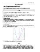
I will now extend my investigation by combining two graphs and finding the gradient at a common point on the two separate graphs, and at the same point on the combined graph. I will use my previously drawn graphs as the separate graphs. I predict that sum of the separate gradients would be equal to the gradient at the common point in the combined graph. If the sum of the separate gradient turns out to be equal to the gradient at that point on the combined graph, I can then say that my gradients are accurate.
The following is the list of graphs, which I am going to make:
Y= -0.5x2 + 0.5x
Y= x2 + 4
Y = x3 – 3x
Graph: Y = 0.5x2 + 0.5x
The table below shows the points, which I have used to plot the graph:
Gradient:
Gradient at point X =-2
Y2-Y1
X2-X1
= -1.7-(4) = 2.56 [rounded to 2.d.p]
-1.5-(2.4)
The table below shows the increment method performed at the point (-2, -3)
(X1, Y1) = -2, -3
(X2, Y2) = -1.999, (-0.5(X2) 2) + (0.5(X2))
(X2, Y2) = (-1.999, -2.9975)
Gradient = Y2-Y1/X2-X1
= -2.9975-(-3)/-1.999-(-2)
= 2.4995 = 2.5 [rounded to 1.d.p]
From the table we can easily see that the gradient at the point (-2, -3) is 2.5
Sum Of Separate Graphs:
Y = -0.5x2 = 1.93
Y = 0.5x = 0.5
Sum = 1.93 + 0.5 = 2.43
Comparison Of Combined Gradients:
From the table above we can see that the gradients are all in close proximity to each other, the slight variations in the gradients occur because the gradients [except that from the increment method] were obtained using the tangent method. I can now conclude that these two graphs were accurate.
Graph: Y = x2 + 4x
The table below shows the coordinates I used to plot the graph:
Gradient:
Gradient at point X =-1
Y2-Y1
X2-X1
= -2-(-4) = 2
-0.5-(-4)
The table below shows the increment method performed at the point (-1, -3)
(X1, Y1) = -1, -3
(X2, Y2) = -0.999, ((X2) 2 + 4(X2))
(X2, Y2) = (-0.999, -2.998)
Gradient = Y2-Y1/X2-X1
= -2.998-(-3)/-0.999-(-1)
= 2.001 = 2 [rounded to 1.d.p]
Sum of separate gradients:
Y = x2 = -2
Y = 4x = 4
Sum = 4 + (-2)
= 2
Comparison Of Combined gradients:
From the table above we can see that the sum of the separate gradients is equal to the combined gradient. This proves that my hypothesis is true. I can now say that the gradients obtained are accurate.
Graph: x3 – 3x
The table below shows the points, which I have used to plot the graph:
Gradient:
Gradient at point X = 2
Y2-Y1
X2-X1
= 5.8-(-1.4) = 9.6
2.4-1.65
The table below shows the increment method performed at the point (2, 2)
(X1, Y1) = 2, 2
(X2, Y2) = 2.001, ((X2) 3 - 3(X2))
(X2, Y2) = (2.001, 2.009006)
Gradient = Y2-Y1/X2-X1
= 2.009006-2/ 2.001-2
= 9.006001 = 9 [rounded to 1.d.p]
Sum of separate gradients:
Y = x3 = 11.33
Y = -3x = -3
Sum = 11.33 + (-3)
= 8.33
Comparison Of Combined gradients:
The table below shows the comparison between the gradients obtained using different methods:
From the table above we can see that again there is variation in the gradients obtained using the different methods. However the most accurate gradient in the table is the one obtained using the increment method [9]. The other method, i.e. the tangent method is quite inaccurate. However since the gradients are in close proximity, I can say that again my prediction was true, but not accurately.
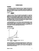
Differentiation
It is possible to find a numerical value for the gradient or rate of change at any point on a curve using this method. The method can be generalised by taking a point P (x, y) on the curve y =f (x). Another point Q is taken very close to P on the curve. The small change in the value of x is δx and the small change in the value of y is δy. The ‘δ’ stands for delta. It is often called the increment (or change) in x and δy is called the increment in y. The gradient of PQ therefore is:
(y + δy) – y = δy
(x + δx) – x = δx
The symbol δy/ δx is called the derivative or the differential co-efficient of y with respect to x. The procedure used to find δy/ δx is called differentiating y with respect to x. I will now carry out the differentiation method for y = x2 and y = -2x2. I will then aim to find a general formula for δy/ δx when y =xn
δy/ δx Function for x2
Taking P as (x, x2) and a neighbouring point Q as [(x + δx), (x + δx) 2] gives:
δy/ δx Function for -2x2
Y = -2x2
Let δy be the increment in y
Let δx be the increment in x
F (x) = -2x2
F (x + δx) = -2 (x + δx) 2
= 2 (x2 + 2x + δx + (δx) 2
Gradient: F (x + δx) – F (x)
(δx) → 0 δx
= -2x2 –4x (δx) –2(δx) 2 +2x2
δx
= -4x (δx) - 2 (δx) 2
δx
Limit δx → 0 = -4x - 2 (δx)
δy/ δx = -4x
So when x = 2 δy/ δx = -8
A general formula for δy/ δx when y = xn
The table below shows the gradient function for all the forms of graphs that I have investigated.
We can now generalise the gradient functions of all the graphs in the form Y = axn. In general when y = x n where n is any real number:
δy/ δx = nx n-1
Thus the gradient function of any graph in the form Y = axn is:
nxn-1