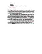
We can estimate the change by looking at graphs of y = x + c, in which the graph is moved very simply along a vertical axis. Increasing c moves the line upwards, decreasing c moves the line down. There are no exceptions to this, fractions and negative numbers will still give the same effect, the gradient never changes. In the graph (right) we can see more clearly how c affects the line y = x + c.
-
If c = 1 then y = x + c will cross the x-axis at 1
The same goes for any other value: y = x + c always crosses the x-axis at c. So by changing constant c it appears that, in this case at least, we are moving the graph up or down by the corresponding value of c. For example, on the left, we can see how graph of y = x + 5 will be moved 5 places upwards from y = x.
From these graphs, we can make a guess at the changes c will have on a more complex graph like
y = ax2 + bx + c. It seems likely that the graph will be moved up and down the y-axis in a similar fashion as before. To find out, we must first fix the values of a and b to reasonable figures, making sure that we are using only one variable. If we use b = 0 and a = 1,
then we still have a quadratic, so this seem sensible.
To the right there are several equations plotted, to give an accurate account of the effects of c. The results were as expected.
Proving observations
We can also prove what is happening to the equation, and whereabouts the y intercept lies (see right and left). In fact, we can also prove a number of other things about
y = x2 + c.
We can also prove that the parabola of
y = x2 + c is symmetrical, and that its line of symmetry will always be along the x-axis. This is shown in the box on the right.
To summarise, we can safely conclude that modifying the constant c moves the graph up or down by the quantity of c (i.e. each point of the parabola has been increase by the value of c). The graph y = x2 + c will always cross the y-axis at c. We can also see that modifying c alone does not affect the gradient of the parabola, nor does it stop it from being symmetrical – the y-axis always being the line of symmetry.
Constant A
Next, we will focus on varying the constant a. We will keep b = 0, and will fix c = 0. If we then start off with a = 1, then we will be given the basic parabola, y = x2. On the same graph, we will plot a as other varying figures, making sure to include minus numbers and fractions.
As we can see, changing a clearly changes the gradient of the curve, except at x = 0 when the gradient will always be 0.. Higher values of a give steeper gradients, fractions give shallower ones. But by how much is the graph affected? To answer this we must begin by measuring the gradient - we can do this one of two ways.
Tangents to y = ax2
By drawing tangents
to the graph at certain
points, we can measure
the gradient of a curve.
Hand drawn tangents
can be inaccurate, however,
when done on a computer
they give reliable gradients.
If we compare the equations y = 2x2 and y = 4x2 we will be able to make a more informative comparison.
First we sketch the graphs, and then draw in a tangent at x = 1. We then measure the gradient of the tangents – for y = 2x2 the gradient at x = 1 is 4. For
y = 4x2 the gradient is 8. In this case at least, we can see that the gradient of the curve has been multiplied by a. To work out if this is true for all cases, we can use calculus.
Calculus
Calculus is an alternative method of working out the gradient of a curve. In situations where tangents can only be hand drawn and may be inaccurate or uneconomical, calculus can be used. The formula for working out the gradient of the curve y = ax2 is 2ax. To see how a changes the gradient of a curve, we will now compare three more equations. We will use a constant (k) value for x, seen as our theory must be general.
y = x2 so gradient is 2 x 1 x k = 2k
y = 3x2 so gradient is 2 x 3 x k = 6k
y = 10x2 so gradient is 2 x 10 x k = 20k
NB: k is any given value of x.
This data also seems to imply that the gradient is simply multiplied by a. We will now try to use calculus to make a general statement.
The gradient at x = k for y = x2 is: 2k
The gradient at x = k for y = ax2 is: 2ak
So in any graph of y = ax2 the gradient at any value of x is equal to the gradient of
y = x2 multiplied by a.
We also know that the graph is always symmetrical, and its line of symmetry is once again always the y-axis from our earlier proofs. However, what happens when we add the constant b into the equation? Does the gradient change or does it remain the same?
Constant B
To examine the effects of constant b, we must once again ‘fix’ the other constants. By fixing a = 1 and c = 0 (giving us the equation y = x2 + bx) we have a quadratic parabola. We may however change a from positive 1 (+1) to negative (-1) because this often affects the way in which the graph moves about the x and y-axis.
Firstly, we can plot several graphs of varying b values and examine the ‘path’ along which y = x2 + bx travels. On the right are two graphs, one depicting the equation with positive values for a, and one with negative.
Graph 1 – Positive A
Here we can see that if we join up the minimum or turning point of each parabola, we form another parabola of the equation y = -x2. This is the ‘path’ of the turning point of y = x2 + bx. Later on, we will show exactly how the equation moves along this path.
Graph 2 – Negative A
With constant a negative, the turning point now moves along the path y = x2 and also moves along it in the opposite direction.
On the next page is a graph portraying how the graph
moves along the path when we modify x.
Path of y = x2 + bx
Gradient of y = x2 + bx
Now that we know how the graph moves, we should measure its gradient. Once again there are two methods of doing so.
Path of y = ax2 +bx
Before we continue, we must note that the path that the turning point moves along when constant b is modified, changes when we modify constant a. Above, we saw that when a is negative, our turning point moves in a different direction along a different path. We will now go into further detail on the turning point of y = ax2 +bx, looking at graphs where a is not only positive or negative, but also a value other than 1 or -1.
On the right is plotted the equation
y = 3x2 – 10x. Here we can see that the turning point does not follow the path y = -x2 as before, when we fixed a as 1, but instead, it now follows the path y = -3x2.
Changing constants A, B and C simultaneously
We will now look at what happens when we change all three constants at the same time, and we will predict what a few graphs involving all three variables would look like. First we will go through several proofs of more precise facts about turning points and x/y intercepts.
We will now go through a step-by-step plotting of a graph, emphasizing any changes each constant might have.
To begin with, we will try to plot the graph of y = 3x2 – 9x + 7. We will first plot the graph y = x2 and then apply our theories about each constant in turn.