Diagram:
HOOK
FORCE METER
BLOCK OF WOOD
SURFACE ON WHICH WOOD IS PULLED ACROSS
Plan:
- The block of wood will be weighed on the balance and its mass will be written down then converted into its weight. This can be done by multiplying its mass by the force of gravity (approximately 9.8N/Kg)
- The block of wood will then be placed at start of the strip of P60E sand paper and the small-scale force meter will then be attached to the hook on the wood. The small-scale meter is more accurate than the large-scale one because you can read off a more accurate result as the values only increase by a small amount each time.
- The force meter will then be pulled slowly while watching it. When the block just starts to move the force observed on the force meter will then be noted. That will be the value found for the static friction for that particular weight.
- Without changing anything the block of wood with the force meter attached to its hook will be placed back at the start of the sand paper. The force meter will then be pulled while watching it carefully so that the wood moves with constant velocity across the sand paper. The force observed on the force meter while the wood is in motion will then be noted. That will be the value found for the dynamic friction for that particular weight.
- Then the block of wood with the force meter attached to it will be placed back at the start of the sand paper. A 100g weight will then be placed on top of the wood and the total mass will then be converted into the total weight and noted.
- Steps 3, 4 and 5 will then be repeated several times until all of the weights have been used, making sure only one is added at a time for each separate set of results. However, if the force required to overcome friction is greater than the small-scale force meter will allow then it will be switched with the large-scale one. All of the results will then be tabulated.
- All of the above will then be carried out a second and third time. This will be done so that there are a large number of results to make averages with. These averages will then be tabulated.
- The whole experiment will the be done a second and third time with the only exceptions that for the second time the P120 sand paper will be used and for the third time the tabletop surface (I will be using the table in the physics practical room) will be used.
- When all of the results have been obtained graphs will be drawn. Two for each different surface (one for static friction and one for dynamic friction) showing static/dynamic friction along the Y-axis and the weight against the X-axis. These will help me in checking my hypotheses. Gradients will then be calculated for each graph, which will be equal to the coefficient of friction for that particular surface (I will explain in detail why in my section entitled ANALYSING RESULTS AND CONCLUSION). This will allow us to see which surfaces need the most force to overcome friction and to compare them.
RESULTS:
Table 1: Results showing the values for static and dynamic friction for certain weights
on the P60E sand paper surface
Table 2: Results showing the values for static and dynamic friction for certain weights
on the P120 sand paper surface
Table 3: Results showing the values for static and dynamic friction for certain weights
on the tabletop surface
ANALYSING RESULTS AND CONCLUSION:
By looking at my results in the above tables, it has been found that as the force holding the two surfaces together (i.e. weight) increases the values for static and dynamic friction increases as well. It has also been found that the values for dynamic friction are less than the values for static friction.
I will only be analysing my average results. The reason being that my average results are probably more accurate as they have been found using numerous results. Therefore the following graphs show the average results for the dynamic/static friction for a particular surface and are plotted showing force against weight.
Trends
The most common trends on my graphs are that as the weight increases so does its corresponding value for static and dynamic friction. It can also be assumed that the static and dynamic friction is directly proportional to the weight as all of my points lie either on or very near the line of best fit, they all show very strong positive correlations. I did some further research and found something called the coefficient of friction. This is a ratio and is defined as how much force in Newtons (N) needs to be applied to a weight of 1N in order for it to overcome friction on a particular surface, it is therefore a constant at all times. It can therefore be concluded that the gradient of a graph is equal to the coefficient of static/ dynamic friction of the particular surface it is representing. This can be seen in the following:
COEFFICIENT OF FRICTION = FRICTION (N)
WEIGHT (N)
GRADIENT = CHANGE IN Y AXIS
CHANGE IN X AXIS
Since the Y-axis represents the force applied, which is equal to the frictional force according to Newton’s Second Law of Motion (see section entitled Background Information), and since the X-axis represents the total weight being exerted on the sand paper, the gradient is therefore equal to the coefficient of friction as long as the units for each axis is in Newtons (N).
The following are gradient calculations and the points I am using have been clearly marked on the graphs. However, since I have multiplied my results for the X-axis by 1000 in order to avoid dealing with small numbers when plotting my graphs I must now divide the results I am using for gradient calculations by 1000 in order for me to use my exact results.
For the graph showing the values found for static friction on the grade P60E sand paper surface:
The X-axis values for the points I’m using are 5500 and 2750 therefore to get the right numbers I must divide them by 1000. So, the values are actually 5.5 and 2.75
GRADIENT = CHANGE IN Y
CHANGE IN X
GRADIENT = 4.8 – 2.4
5.5 – 2.75
GRADIENT = 2.4
2.75
GRADIENT = 0.873 (to 3 d.p)
So, this means that for every 1N of weight a force of 0.873N has to be applied to it in order for it to overcome static friction in the case of wood on grade P60E sand paper. Hence, the coefficient of static friction of wood on P60E sand paper is approximately 0.873 according to its definition.
For the graph showing the values found for dynamic friction on the grade P60E sand paper surface:
The X-axis values for the points I’m using are 6000 and 3000 therefore to get the right numbers I must divide them by 1000. So, the values are actually 6 and 3
GRADIENT = CHANGE IN Y
CHANGE IN X
GRADIENT = 4 - 2
6 – 3
GRADIENT = 2
3
GRADIENT = 0.667 (to 3 d.p)
So, this means that for every 1N of weight a force of 0.667N has to be applied to it in order for it to overcome dynamic friction in the case of wood on grade P60E sand paper. Hence, the coefficient of dynamic friction of wood on P60E sand paper is approximately 0.667 according to its definition.
For the graph showing the values found for static friction on the tabletop surface:
The X-axis values for the points I’m using are 8500 and 6000 therefore to get the right numbers I must divide them by 1000. So, the values are actually 8.5 and 6
GRADIENT = CHANGE IN Y
CHANGE IN X
GRADIENT = 4 – 2.8
8.5 – 6
GRADIENT = 1.2
2.5
GRADIENT = 0.48
So, this means that for every 1N of weight a force of 0.48N has to be applied to it in order for it to overcome static friction in the case of wood on the tabletop surface in my physics practical room. Hence, the coefficient of static friction of wood on the tabletop in question is approximately 0.48 according to its definition.
For the graph showing the values found for dynamic friction on the tabletop surface:
The X-axis values for the points I’m using are 6500 and 1050 therefore to get the right numbers I must divide them by 1000. So, the values are actually 6.5 and 1.05
GRADIENT = CHANGE IN Y
CHANGE IN X
GRADIENT = 2.4 – 0.4
6.5 – 1.05
GRADIENT = 2
5.45
GRADIENT = 0.367 (to 3 d.p)
So, this means that for every 1N of weight a force of 0.367N has to be applied to it in order for it to overcome dynamic friction in the case of wood on the tabletop surface in my physics practical room. Hence, the coefficient of dynamic friction of wood on the tabletop in question is approximately 0.367 according to its definition.
For the graph showing the values found for static friction on the grade P120 sand paper surface
The X-axis values for the points I’m using are 6500 and 1750 therefore to get the right numbers I must divide them by 1000. So, the values are actually 6.5 and 1.75
GRADIENT = CHANGE IN Y
CHANGE IN X
GRADIENT = 5.16 – 1.4
6.500 – 1.75
GRADIENT = 3.76
4.75
GRADIENT = 0.792 (to 3 d.p)
So, this means that for every 1N of weight a force of 0.792N has to be applied to it in order for it to overcome static friction in the case of wood on the grade P120 sand paper surface. Hence, the coefficient of static friction of wood on the grade P120 sand paper is approximately 0.792 according to its definition.
For the graph showing the values found for dynamic friction on the grade P120 sand paper surface
The X-axis values for the points I’m using are 5500 and 1500 therefore to get the right numbers I must divide them by 1000. So, the values are actually 5.5 and 1.5
GRADIENT = CHANGE IN Y
CHANGE IN X
GRADIENT = 3.6 – 1
5.5 – 1.5
GRADIENT = 2.6
4
GRADIENT = 0.65
So, this means that for every 1N of weight a force of 0.65N has to be applied to it in order for it to overcome dynamic friction in the case of wood on the grade P120 sand paper surface. Hence, the coefficient of dynamic friction of wood on the grade P120 sand paper is approximately 0.65 according to its definition.
Table 4: Table of Gradients
From the above table it can clearly be seen that the values for dynamic friction are less than the values for static friction. This is because the gradients found for the graphs showing dynamic friction for a particular surface are less than the gradients found for the graphs showing static friction for a particular surface. It can also be seen from the above table that the grade P60E sand paper surface has the highest values for friction and that the tabletop surface has the lowest values for friction.
How my results support or undermine my original predictions
1. I predicted that the heavier the object is when on a particular surface the more force would be required to overcome friction. This has been proven true as the graphs clearly show a very strong positive correlation.
2. I also predicted that the static and dynamic friction would be directly proportional to the weight of the object pressing down onto the surface. This has also been proven true as nearly all of my points, except for a few that are probably anomalous results anyway and which I shall talk about in my EVALUATION section; lie either near or on the line of best fit.
3. I said that the values, which I would find for dynamic friction, would be less than my values found for static friction. This has been proven true, as the gradients for the graphs showing dynamic friction are less than the gradients for the graphs showing static friction.
4. I also said that the grade P60E sand paper would have the highest values as when I touched it seemed to be the roughest surface out of all of them whereas the tabletop surface seemed to be the smoothest and so should have had the lowest values. This has been proven true as the gradients for the graphs showing dynamic and static friction for the grade P60E sand paper are higher than those on the graphs for the tabletop surface in my physics practical room.
5. I thought that my graphs would look like the ones I did in the section entitled PLANNING. This seems to be the case as I found that all of the graphs I did bear resemblance to these graphs.
Conclusion
The heavier an object is when on a particular surface the more force is required to overcome friction. It can also be said that the static and dynamic friction are both directly proportional to the weight of the object pressing down onto a surface. This is because, as explained in my predictions earlier, the coefficient of friction should stay constant no matter what the weight is. Therefore as the weight increases the dynamic and static friction should increase as well.
It has also been seen that the values, found for dynamic friction, are less than the values found for static friction on a particular surface. I can explain this because when an object is moving it has momentum and therefore less force needs to be exerted on it in order to keep that motion. However, when an object is at rest it has no momentum and therefore more force is needed to get it in motion. And according to Newton’s Second Law of Motion the forward force is equal to the frictional force, so, if less force is needed to keep an object in motion, the frictional force (in this case dynamic friction) therefore will be less as well.
In this particular case it was possible to guess which surfaces would have the highest values of friction by touching them. However, this won’t always be the case as in some situations the surfaces may only have minor differences in the surface structure. This makes it impossible to guess, by using your sense of touch, which one will have the highest values of friction.
Overall, in this experiment, it has been found that the surface with the most friction was the grade P60E sand paper with a coefficient of static friction of approximately 0.873 and a coefficient of dynamic friction of approximately 0.667. The next surface with the most friction was the grade P120 sand paper with a coefficient of static friction of approximately 0.792 and a coefficient of dynamic friction of approximately 0.65. Finally the surface with the least friction in this experiment was the tabletop surface in my physics practical room with a coefficient of static friction of approximately 0.48 and a coefficient of dynamic friction of approximately 0.367. However these are only approximate results, as I don’t think my experiment was accurate enough to give definite results, the reasons for this can be found in my next section entitled EVALUATION. Furthermore, even a monomolecular layer of some surface impurity affects the experimental results.
EVALUATION
In my investigation I was pleased with my achievements. The procedure I used to carry out the experiment seemed to be suitable and good, as my results appeared to be very accurate in respect to my predictions. However I did get some anomalous results that can be seen on my graphs as I have identified them with the help of my percentage error calculations just below and encircled them.
I will now calculate the percentage error of all points that do not lie on the line of best fit for each graph. This will show to what extent my results are incorrect and will be carried out by using the following formula and my graphs:
ΔX * 100 = % Error
X
In the formula above, ΔX represents the distance of the point away from the best line of fit and X the actual y-coordinate of where the point is meant to be. I will only call one of my results anomalous if it has 7.5 % or more percentage error as I feel that this is a reasonably high percentage error.
For graph 1:
Point 2:
% ERROR = Δ X * 100
X
% ERROR = 0.14 * 100
2.24
% ERROR = 6.25 %
Point 3:
% ERROR = Δ X * 100
X
% ERROR = 0.11 * 100
3.08
% ERROR = 3.57 % (3s.f)
Point 4:
% ERROR = Δ X * 100
X
% ERROR = 0.08 * 100
3.92
% ERROR = 2.04 % (3s.f)
Point 5:
% ERROR = Δ X * 100
X
% ERROR = 0.18 * 100
4.8
% ERROR = 3.75 %
Point 6:
% ERROR = Δ X * 100
X
% ERROR = 0.22 * 100
5.64
% ERROR = 3.90 % (3s.f)
Point 8:
% ERROR = Δ X * 100
X
% ERROR = 0.14 * 100
7.36
% ERROR = 1.90 % (3s.f)
For graph 2:
Point 1:
% ERROR = Δ X * 100
X
% ERROR = 0.04 * 100
1.04
% ERROR = 3.85 % (3s.f)
Point 2:
% ERROR = Δ X * 100
X
% ERROR = 0.2 * 100
1.7
% ERROR = 11.8 % (3s.f)
Point 3:
% ERROR = Δ X * 100
X
% ERROR = 0.07 * 100
2.34
% ERROR = 2.99 % (3s.f)
Point 4:
% ERROR = Δ X * 100
X
% ERROR = 0.10 * 100
2.98
% ERROR = 3.36 % (3s.f)
Point 5:
% ERROR = Δ X * 100
X
% ERROR = 0.14 * 100
3.64
% ERROR = 3.85 % (3s.f)
Point 6:
% ERROR = Δ X * 100
X
% ERROR = 0.07 * 100
4.3
% ERROR = 1.63 % (3s.f)
Point 7:
% ERROR = Δ X * 100
X
% ERROR = 0.71 * 100
4.46
% ERROR = 15.9 % (3s.f)
Point 8:
% ERROR = Δ X * 100
X
% ERROR = 0.09 * 100
5.58
% ERROR = 1.61 % (3s.f)
For graph 3:
Point 1:
% ERROR = Δ X * 100
X
% ERROR = 0.02 * 100
0.73
% ERROR = 2.74 % (3s.f)
Point 2:
% ERROR = Δ X * 100
X
% ERROR = 0.12 * 100
1.2
% ERROR = 10 %
Point 3:
% ERROR = Δ X * 100
X
% ERROR = 0.08 * 100
1.65
% ERROR = 4.85 % (3s.f)
Point 4:
% ERROR = Δ X * 100
X
% ERROR = 0.2 * 100
2.1
% ERROR = 9.52 % (3s.f)
Point 5:
% ERROR = Δ X * 100
X
% ERROR = 0.11 * 100
2.58
% ERROR = 4.26 % (3s.f)
Point 8:
% ERROR = Δ X * 100
X
% ERROR = 0.21 * 100
3.96
% ERROR = 5.30 % (3s.f)
For graph 4:
Point 1:
% ERROR = Δ X * 100
X
% ERROR = 0.02 * 100
0.59
% ERROR = 3.39 % (3s.f)
Point 2:
% ERROR = Δ X * 100
X
% ERROR = 0.06 * 100
0.94
% ERROR = 6.38 % (3s.f)
Point 3:
% ERROR = Δ X * 100
X
% ERROR = 0.05 * 100
1.3
% ERROR = 3.85 % (3s.f)
Point 4:
% ERROR = Δ X * 100
X
% ERROR = 0.13 * 100
1.66
% ERROR = 7.83 % (3s.f)
Point 5:
% ERROR = Δ X * 100
X
% ERROR = 0.27 * 100
2.2
% ERROR = 12.27 % (3s.f)
Point 6:
% ERROR = Δ X * 100
X
% ERROR = 0.3 * 100
1.98
% ERROR = 15.2 % (3s.f)
Point 7:
% ERROR = Δ X * 100
X
% ERROR = 0.12 * 100
2.74
% ERROR = 4.38 % (3s.f)
Point 8:
% ERROR = Δ X * 100
X
% ERROR = 0.13 * 100
3.1
% ERROR = 4.19 % (3s.f)
For graph 5:
Point 1:
% ERROR = Δ X * 100
X
% ERROR = 0.09 * 100
1.24
% ERROR = 7.26 % (3s.f)
Point 2:
% ERROR = Δ X * 100
X
% ERROR = 0.1 * 100
2
% ERROR = 5 %
Point 3:
% ERROR = Δ X * 100
X
% ERROR = 0.08 * 100
2.78
% ERROR = 2.88 % (3s.f)
Point 5:
% ERROR = Δ X * 100
X
% ERROR = 0.06 * 100
4.34
% ERROR = 1.38 % (3s.f)
Point 6:
% ERROR = Δ X * 100
X
% ERROR = 0.33 * 100
5.9
% ERROR = 5.59 % (3s.f)
Point 7:
% ERROR = Δ X * 100
X
% ERROR = 0.17 * 100
5.14
% ERROR = 3.31 % (3s.f)
Point 8:
% ERROR = Δ X * 100
X
% ERROR = 0.52 * 100
6.68
% ERROR = 7.78 % (3s.f)
For graph 6:
Point 1:
% ERROR = Δ X * 100
X
% ERROR = 0.04 * 100
1.04
% ERROR = 3.85 % (3s.f)
Point 2:
% ERROR = Δ X * 100
X
% ERROR = 0.06 * 100
1.66
% ERROR = 3.61 % (3s.f)
Point 4:
% ERROR = Δ X * 100
X
% ERROR = 0.16 * 100
2.84
% ERROR = 5.63 % (3s.f)
Point 5:
% ERROR = Δ X * 100
X
% ERROR = 0.07 * 100
3.6
% ERROR = 1.94 % (3s.f)
Point 7:
% ERROR = Δ X * 100
X
% ERROR = 0.02 * 100
4.88
% ERROR = 0.410 % (3s.f)
Point 8:
% ERROR = Δ X * 100
X
% ERROR = 0.08 * 100
5.5
% ERROR = 1.45 % (3s.f)
Table 5: Table of Percentage Errors for each Graph
As can be seen from the above table, there are quite a few of what I would consider to be anomalous results (i.e. 7.5 % or higher percentage error). The most accurate graphs appear to be graphs 1 and 6 as they have no anomalous results and the least accurate seems to be graph 4 as it has three anomalous results. Graphs 2 and 3 have two anomalous results and graph 5 has only one anomalous result. So the best results were obtained from the P120 sand paper surface (graphs 5 and 6) with only one anomalous result present and the worst results were obtained from the tabletop surface (graphs 3 and 4) with a total of five anomalous results present.
If the experiment is looked at as a whole, the weights used don’t really seem to affect my results as my anomalous ones seem to have occurred just as many times with the lighter weights as they have with the heavier ones. However, if the above table is looked at more closely it can be seen that the worst results found overall were the ones represented on the graphs by points 2 and 4 which were found using weights of 2.548 N and 4.508 N.
To improve the reliability of the evidence I would take more results, especially for the tabletop surface and for the weights of 2.548 N and 4.508 N which were used, as these were the things in my experiment which contributed the most to obtaining anomalous results.
I don’t think that the evidence found in my experiment is sufficient to support a firm conclusion. Even though I think my results are accurate enough to show me correct patterns and trends, there are things apart from my anomalous results such as the coefficients of friction I have found for the wood on the surfaces I have used, which I feel aren’t very accurate. The reason being that when I was reading force measurements off of the force meter it would fluctuate, so I had to take an intelligent guess of what the values were. Therefore if any of these results were wrong they in turn would make my graphs wrong and hence my conclusion incorrect.
Further Work
To improve the experiment in order to provide additional and more reliable evidence for a conclusion I would carry out the experiment as shown in the following diagram:
PULLEY
FORWARD FORCE
WOODEN BLOCK RESTING ON A HORIZONTAL
SURFACE
SCALE-PAN
This experiment doesn’t involve using a force meter; therefore, readings will be easier to take. Firstly, to find the value of static friction, the block’s mass is found by weighing it and then converted into its weight. Then, small masses are added, one at a time, to the scale-pan in order to increase the forward force. Eventually a point is reached at which the block starts to slide, and then the total mass that was placed in the scale-pan is converted into the total weight. This will be the value for the forward force and hence, by knowing this, the static frictional force can be found according to Newton’s Second Law of Motion which I have explained how to do in my section entitled BACKGROUND INFORMATION. Once this has been found, the coefficient of static friction can be found for wood on this particular surface as well. For dynamic friction, the experiment is carried out in almost the same way with the exception that the block is given a slight push each time a mass is added to the scale-pan. The value of the forward force at which the block continues to move with constant velocity after being pushed is the value of the dynamic frictional force. Once this has been found, the coefficient of dynamic friction can be found for wood on this particular surface as well.