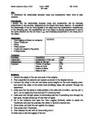
Organizing and presenting raw data:
NOTE: For Average Acceleration, it is considered to be digital error. Which rounded of the last digit.
For example:
If the machine shows to 2 decimal points, 3.14 then the uncertainties for this are ±0.005 as the range of the data could go from 3.135 to 3.145.
As we could see that the data above [average acceleration] is all rounded up to 3s.f. And some has 2 decimal points, 3 decimal points and even 4 decimal points so the uncertainties may differ of 0.005, 0.0005 or 0.00005. But if we look closely only one of them is with 4 decimal points and the majority is with 3 decimal points, therefore I come up that the uncertainties for average acceleration is ±0.0005.
Summary of all the Error Uncertainties
We used 10 weights. Each weight’s uncertainty is 0.005g.
And total uncertainty is 10 x 0.005 = ± 0.05g.
For example:
Cart and Hook + 8 weights = ± 0.005 + 9 x ± 0.005
= ± 0.05g
Remember that this is the total uncertainty, which are the total mass’s uncertainties. But while you are doing addition the uncertainty are being added together. Since there are two things added therefore the uncertainty for each is now ± 0.025.
While since “g” has no uncertainty and now that I have said that the uncertainty for the mass hanging is ± 0.025, therefore there is no change in uncertainty during the multiplication is done.
Graph Data of x and y axis:
NOTE: The uncertainties are too small to be drawn onto the hand drawn graph, and will not be seen with our bare eyes if drawn, therefore it is irrelevant for me to draw it.
Theory:
Isaac Newton described the relationship of the net force applied to an object and the acceleration it experiences in the following way:
the acceleration (a) of an object is directly proportional to and in the same direction as the net force (Fnet), and inversely proportional to the mass (m) of the object.
Firstly my investigation is based around the formula of F = ma. In the set-up that I am using the only factor that is constant is the force applied.
From this you can tell something about the proportionality between the other two factors, the 1/mass and the acceleration. That is that they are directly proportional, and this is stated in Newton's laws of motion. You can tell proportionality on a graph because of two features:
1.The graph is a straight line
2. The line goes straight through the origin
We also know that when the graph has been drawn we will be able to take the gradient of the line. This gradient should be equal to force applied:
F = ma
a = F / m
= F (1/m)
Overall I state that when 1/mass is plotted against acceleration then the graph will be directly proportional. Then if I take the gradient of the graph then it should equal the force applied [which is constant].
Electronic Graph:
Graph Analysis:
Through my working I have been able to draw a graph of 1/mass against acceleration for which, as I have previously stated, the gradient would be the force applied. I did find that as the mass of the cart increases then the subsequent acceleration of the mass (cart) would also increase. The graph shows the average results for 1/mass against acceleration. The main point that I have focused on so far is that when this graph is plotted, because of its direct relation to the formula F = ma, the graph shows the following a = F (1 / m). This means that when the gradient of the straight line is taken (for this is a graph of proportionality) the gradient will equal the force on hook. I, indeed, did measure the gradient of the graph (which should have been 0.488 ± 0.025 N).
In fact gradient of the graph is 0.411N which is 0.077N away from the actual force on hook. There must be another force acting that I have so far, which is friction and air resistance.
Friction is a force that opposes the movement of an object, and it acts in the opposite direction to the way the object is moving. Between two surfaces it depends on:
- the type of surface
- the size of the reaction force.
Air resistance is a special type of frictional force, which acts upon objects as they travel through the air. Like all frictional forces, the force of air resistance always opposes the motion of the object. And the three main factors of air resistance are:
1. Aerodynamic [streamline] properties of the object
2. Density of the object
3. Velocity of the object
The more aerodynamic, dense, and fast the object is, the less air resistance there is as compared to the force of the accelerating object. For example:
If you used a heavier metal, for example lead, instead of other stuff like plastic, then it would be relatively smaller (if both have same mass). And if you attach more mass on the hook, then you would have a greater acceleration, so it goes at a greater velocity, so then less air resistance.
From these facts I can begin to understand why my graph looks the way it does. Also, if looked at closely, the line of the results does not go through the origin of the graph. This tells me that, just like activation energy is needed to be overcome before a chemical reaction can occur, a force is needed to provide an initial 'jump-start'. This accounts for the 'error' in reading at the start, but still there is an error in the overall gradient of the graph.
Conclusions:
Overall my results were not as I would have expected them to be, but I had provided sufficient reasons for this. From the theory I know that 1/mass is directly proportional to acceleration, although my result from the graph shows 0.411N, and the original value is 0.488 ± 0.025 N, therefore the result is still accepted as it is still within the range of the error uncertainty.
Plus I had explained the caused of friction and air resistance acting on this experiment affected the time taken to be longer as friction acts opposite direction to the object therefore causing a longer time to travel.
Therefore I can conclude that friction and air resistance must be acting at all times during the experiment (after all there is still a straight line which means consistency throughout the testing). So I conclude that the experiment is a fair test.
Evaluation:
Although my results were the readings that I expected to take, I was very happy indeed with the procedure and the way in which I still managed to maintain fair conditions for it to take place. But there were also some weaknesses in the procedure. The range of testing (s) is too small; the highest and the lowest only differ by 4kg, which is way too small. From my result, we couldn’t know at 10kg, if it is going to be still the same. Plus, for each testing point, the experiment should have been repeated for more than 5 times, thus allowing for greater accuracy in results but it will be better to do it as many as we can.
This leads me on to the point that, although I did not take friction and air resistance into account, my results were still congruent and they still followed the pattern that I expected and still followed the trends of the graphs that I included in my hypothesis. This is shown by the fact that my best-fit line on graph, despite having an inaccurate gradient, had the points plotted very close to it. Also my readings did not show up any anomaly results, therefore the results recorded should be fairly accurate.
Modifications:
Of course if I did indeed do the experiment again I would have to take friction and air resistance into account. The way in which I would suggest to overcome this would be to use an air track. This would get rid the experiment most of friction though due to it being an air track there would still be some resistance from air molecules. Though this method, if one does not already own an air track, would be an expensive method. But in this method you will encounter air resistance as well as a little bit of friction. But nothing could be done about the air resistance problem in this experiment due to the equipment and place to be done in the school laboratory.
However, the error may be reduced significantly if a greater range of testing for weights (kg) was used.
For example, tests can be made from 0.01kg and with intervals of 0.001kg for 20 (or even more) testing points.
Plus, to decrease the error or chances of getting unreasonable results, 7 (or more) runs should be performed for each testing point.
By increasing the range and repetition of testing may bring results closer to the literature value which will let F = ma, where the gradient will be closer to the force applied.