The point of this model is a fundamental one, deviations in gene frequencies from this model are due to evolutionary forces as it has been shown that is the assumptions are met the system self perpetuates. Hence it makes a good null hypothesis model for which to test population genetics.
Deviations from Equilibrium.
Changes in allele frequencies are fuelled by evolutionary forces, of which there are five. Three of which, mutation recombination and migration, create variance in the genes, providing the raw material for genetic drift and natural selection act upon and alter their frequency in the population.
Mutations
Mutations that alter gene frequencies in populations occur at a molecular level from incorrect DNA replication in the gametes produced by the individuals. Improper pairing of bases leads to daughter strands containing a different genetic code to their parental genome. Although it is vital in evolution, the rate at which mutation occurs is very small, in most eukaryotic nuclear DNA 1 x 10⁻⁹ substitutions occur per site per year. Even if there is a site substitution, the chances of it having an effect are even slimmer as firstly it has to occur within the 20% coding part of the genome and secondly it has to bypass the redundancy of the genetic code, altering the codon to read for another amino acid. These are called non-synonymous mutations; the only type that confers a genetic variation on the organism for natural selection or drift to work on. The mutations that are degenerate to the amino acid sequence are assumed to be neutral, unable to be effected by evolutionary forces, are called synonymous mutations. However there is evidence that they may impart some alteration in fitness, for example codon bias in drosophila. Because the mutation rate is so low, it is usually a weak force for changing allele frequencies alone. The other two sources of genetic variation play an important part in creating the variation seen today.
Recombination and migration can also be seen as mutations, but on a much larger scale (entire genes are changed/mutated from one allele to another). Recombination occurs during the first meiotic division of gametes, resulting in an exchange of genes between homologues. This does not alter the allele frequencies in the population but it “shuffles” genes along chromosomes resulting in new allele combinations to their parents. These new allele combinations can then be acted upon by the forces of evolution. Migration involves the influx of new alleles into the population that have been shaped by different evolutionary forces. An example of migration could be seen in America where there is on average a 3.5% gene flow between American black and American white populations per generation.
Hence latter two forces resolve the problem regarding the slow rate of mutation in the genome and the huge amount of variation in population seen today. They are also much safer forms of altering the genetic frequencies of a population as they have already been “run in” by other members of the population or species unlike a random mutation which is much more likely to have a deleterious effect.
However none of the above forces of evolution are strong enough to alter the gene frequencies of a population and so two additional forces are used to describe how the variations created can alter the structure of the allele frequencies in the population. These are random genetic drift and natural selection.
Random Genetic Drift
Random genetic drift alters allele frequencies by chance, in a random fashion. The random fluctuations in allele frequency rely mainly on the fact that the number of combinations of gametes that are produced by and individual greatly outnumber the amount of individuals produced in the next generation. In other words a lot of alleles don’t make it into the next generation merely due to sampling error. The ones that do are randomly selected from the allele pool but they contribute directly to a change in the allele frequency in the next generation.
There is a model for the time it takes for an allele to be fixed (p or q =1) and it is a powerful tool for population geneticists as it enables them to see what effect random drift has on populations as a force of genetic variation. The number of alleles in a diploid population is 2N, therefore assuming random assortment, mating and no new mutations (also that N=Ne) the probability of any allele reaching fixation is 1/2N and the time it would take for it to do so is approximately 4N with large error bars either side. From this model you can see that the size of the population will have an effect on how much genetic drift will affect allele frequencies. This is well illustrated with this graph (Li 1998);
This clearly illustrates that genetic drift is much more important when population sizes are small, due to 1/2N being a lot more favourable for any given allele. Smaller populations obtain fixation much faster whereas larger populations see drift take a lot longer to fix an allele. This model assumes that all alleles are equal in terms of conferring fitness to their host, so neutral mutations are the most likely to be fixed (note this is not the same as synonymous mutations as this regards whether they impose a selective advantage on the individual not a neutral change in the amino acid code). However advantageous alleles can be lost by genetic drift if they are in small enough frequencies, but they cannot be fixed by drift as they undergo the final evolutionary force natural selection.
Natural Selection
If non-synonymous mutations arise a new allele is created. This will in some way, no matter how small, alter the performance of the gene product and distinguish it from other alleles. This difference will effect how the individual performs in reproductive fitness by either hindering it enhancing it, or in small differences no change will be conferred. Therefore gene frequencies will shift in a particular direction favouring the line of increased fitness (adaptation to the environment). This is due to those individuals with advantageous alleles contributing more to the next generations’ allele pool. The converse is also true, deleterious alleles will be removed from the population as they are unable to contribute as much to the next generation as they have reduced fitness. The process of natural selection therefore differs to genetic drifts’ random contribution to the next generation in being a selective contribution to the next generation causing a directional change in allele frequencies.
Natural selection however does not usually act at the level of individual loci (specific disease resistance may be an exception), rather the entire phenotype is put under selection pressures so some advantageous alleles may never alter gene frequencies because they have other deleterious alleles present of are lost through drift. Overall phenotype fitness is a more important factor than individual allele fitness.
The types of shift produced by natural selection in response to the environment allow for even greater variation in the distribution and frequency of genes in a population. The following is a description of the different type of selection, both on the individual loci and how it manifests itself in phenotypic selection.
From these examples it is clear that the modes of selection that increase the amount of variation in the population and hence drive evolution are Positive and Disruptive selection.
The discussion on how variation is altered in populations would not be complete without a mention of the Evolutionary Geneticists “Great Obsession” (E Holmes 2000), that is what proportion of alleles in the population are due to drift (Neutralist) and what are due to selection (selectionist). I could write an entire essay on the debate but it appears that the neutralist theory is the most accepted nowadays. This states that the majority of mutations are either neutral of deleterious. Natural selection acts upon the deleterious mutations and also the very few advantageous mutations, but is more of a purifying force rather than an adaptive positive force whilst mutation and genetic drift are the main forces in molecular evolution (Kimura 1983).
Measurement of Genetic Variation and Quantitative Genetics
All of these underlying theories are useful but in order to be of any use they must be tested and the genetic variation of populations must be determined using experimental techniques. Here is a summary of the different types of procedures that can be performed and the types of information they reveal about genetic variation.
Visual inspection was the first assay used for assessing the amount of variation within a population. Looking at the different phenotypes gave an indication of the diversity seen, but this was a very qualitative assay as it was impossible to differentiate between the phenotypes that were caused by genetic factors and those caused by environmental ones. It was clear that a quantitative assay which produced results that could be statistically analysed was needed.
Allozyme analysis and Heterozygosity.
This was the first biochemical assay for genetic variation within a population. Allozymes are distinct forms of enzymes encoded by different alleles at a single locus. These enzymes differ in charge and can be separated from each other on a gel using SDS gel electrophoresis, accumulating in different bands according to their charge (electrophoretic mobility). If the proteins of interest are collected from a sample of different individuals and run on a gel then an indication of the genetic variation within the population can be seen, through the number of bands obtained. This was a very limited method as firstly it was restricted to enzyme genetic variation within a population and as with all protein work, obtaining a pure enough sample is hard enough, let alone creating the probes and antibodies needed to specifically identify it.
However analysis of allozyme variation is the backbone of modern population genetics, as it provided real data to perform analysis on for genetic variation. The allele frequencies p and q are a very simple description of the amount of genetic variation in a population, and they get less informative and cumbersome as the number of alleles increases. Therefore what allozymic analysis allowed population geneticists to do was assess the overall frequency of heterozygotes in the population Heterozygosity (h), equivalent to the probability that any two alleles (not necessarily from the same loci) sampled randomly in the population are different. (h) will be greatest when there are many alleles, all at equal frequency. It is also possible to calculate Average Heterozygosity (H) which gives the average number of heterozygotes per locus.
DNA Sequence analysis and Segregation, Pairwise and Nucleotide Diversity.
The development of molecular tools greatly enhanced the accuracy and resolution obtained in population genetics. For the first time an unambiguous element could be used for comparisons within and among populations and across taxa. DNA analysis is also more informative because it doesn’t rely on the presence or purification of proteins and mutations can be studied at the base level therefore realising synonymous mutations. Current methods of using DNA analysis are comparing genome sequences for similarities and the use of molecular markers. These molecular markers are sections of DNA that are highly polymorphic in a population. These sections can be analysed and then compared to other individuals in the population to get an indication of the diversity. The markers most commonly used are areas of rapidly evolving DNA; otherwise there would not be enough variation for analysis in a population due to the low rate of mutation.
Micro satellites and Mini satellites are short sections (30-40bp and 2-4bp respectively) of highly repetitive DNA. They are non-coding and therefore are not put under strong functional constraints so they are free to mutate and evolve fairly rapidly, 1 in105 substitutions per site per year. The number of repeated sections is key to the polymorphism as errors occur in the proof reading mechanisms during DNA replication when it is highly repetitive. This will once again give you a distinct banding pattern between individuals and provides data to perform Heterozygosity tests and if the sections are sequenced some of the other tests.
Perhaps the simplest and most informative method of obtaining an index of genetic diversity is to compare a sequence data from a variety of sources, looking for individual nucleotide substitutions, Single Nucleotide Polymorphisms (SNPs). This is calculated as the number of segregating sites (i.e. polymorphisms), S. However like (h) it is more informative to know about the average number of segregating sites per nucleotide. This is found by simply dividing the number of segregating sites by the length of the DNA sequenced (L). Another frequently used measure is the average number of pairwise nucleotide differences between sequences ( ∏ ). This looks at the amount of variation in sequence data between samples. This differs from S because it looks at the actual nucleotide differences rather than the number of sites that are able to have nucleotide differences. Once again this statistic can be standardised by dividing by L to give you the average number of bases per nucleotide, or the nucleotide diversity, π.
One final measure of population diversity is called θ, which is equal to 4Neμ. θ is important as it describes the amount of variation per site if the genes were evolving entirely under neutral evolution. This is important as it allows testing against the neutral theory of evolution. However it does contain two parameters that are difficult to measure accurately and the reason for the “great obsession” was partly due to the fact that both hypotheses were difficult to unambiguously test. Obtaining Ne is possible in a population although the error bars are high, but accurately defining the mutation rate in molecular terms is much harder because, as we have seen, there are variable rates depending on the type of genomic DNA you use.
Quantitative genetics is an important field to population geneticists as it deals with the amount of variation in the population that is due to genetic factors and how much is attributable to the environment. The variability (V) of the organism is modelled as VG(enetic) + VE(nvironmental) = VP(henotype). Assessment of this is important as it provides information as to how much variation is heritable. Heritability can be assessed in two ways one being Broad Sense Heritability (H2) which is the proportion of variation in a character that is genetic (also VG). Narrow Sense Heritability (h2) works by splitting VG into three components, the amount of variation due to gene interactions (epistasis), variation due to dominant interaction (i.e. codominance) and assessing the amount of variance that is attributable to the individual additive effects of genes (i.e. A and a confer different traits). The additive variance is important here as it is the only type of variance artificial selection can work on.
Practical Uses Of Population Genetics
There are many examples of uses for population genetics, some of which I have already touched upon. Hopefully I have highlighted in this essay the most important role population genetics has played is in the field of evolutionary biology, where it’s methods and models are able to test theories governing the driving forces of evolution. Without population genetics there would be no science behind evolution, just a collection of conjecture and interesting “just so” stories.
Commercial uses of population genetics have just been mentioned, concerning artificial selection in agriculture. Although this has been performed for thousands of years without knowledge of sequence data or heritability, the science has made the selection process a lot more efficient and this results in a higher productivity and capitol return.
Using population genetics in recent years has become increasingly important in the medical field. Genetic diseases can be identified through the techniques used to study individual genetic variation and it is possible to find carriers and take appropriate steps to reduce the incidence of the disease. Also the modelling behind the genetic variation within a population allows governments to assess what screening procedures it needs to perform as an offset to the cost of treating individuals and the overall cost to the fitness of the population. An interesting example is found concerning the incidence of Taysachs. Taysachs is an autosomal recessive disease and can be identified by looking at the activity of Hexosominidase A. The local government wanted to see if it was feasible to screen the population for carriers to reduce the costs of treatment on the health service. The cost would have been $2x10⁷ to screen the population and the chances of carriers mating is one in 107 and even then the chances of producing a homozygote were 1 in 4. Simple economics ruled out the possibility of a population wide screen for carriers. However using population genetics a small sub population, the Ashkenazi Jews, were identified as having an abnormally high incidence of the disease 1 in 30. By screening only the females in that population, and then male partner if a carrier identified, it turned out to be economically feasible to screen this population and within a single generation the incidence of the disease was reduced 95%. (D Roberts 2001 Lecture).
Although this is only a brief summary of what population genetics can do for us, it illustrates that its usefulness extends beyond that of proving hypothesis and can be used to have a positive impact on people’s lives. Population genetics will become increasingly important over the next few decades as models and methodology is refined and the applications for this tool will become increasingly widespread.
Bibliography
Page & Holmes (1998) Molecular evolution: a phylogenetic approach. Blackwells.
Li (1997) Molecular evolution. Sinauer Associates.
Ridley (1996) Evolution. Blackwells.
Li & Graur (1991) Fundamentals of molecular evolution. Sinauer Associates.
Maynard-Smith (1989) Evolutionary genetics. Oxford University Press.
Kimura (1983) The neutral theory of molecular evolution. Cambridge University Press.
Lecture notes from
D. Roberts TT1 2001
E. Holmes MT2 2001