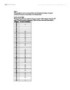
From the above table C.I - 10 (of 100 weights) Mean, Median, Mode and Standard Deviation by using same above mentioned formulas.
Hence,
Mean: 61.6
Median: 50.5
Mode (marked in yellow): 55
Standard Deviation: 31.17594522
**From these calculations (above) we can clearly see that the mean obtained is not the same as the mean calculated when all the 100 weights are taken at a time, this is because in the above calculations we have divided it into class intervals (i.e. 10). This shows as that when the data is arranged in a different class interval range it gives us a different mean.
From the same table (of class interval 10), the graph (between Frequency & Middle Value of Weights) obtained was:
A very important thing that should be taken into consideration is that according to the mean calculated above was 61.6 is not the same as the one which we obtain by looking at the graph (i.e. 55.32) since, in the graph there is a certain minor fall (i.e. at 80 - 90) this is because, at that certain class interval there are very less people with that certain weight.
After the first graph was made for a class interval of 10, I proceeded to do a second graph with a lower class interval (i.e. 5, shown bellow) in order to reduce the difference in mean (by following the same procedure as the class interval of 10).
From the above table C.I - 5 (of 100 weights) I calculated the Mean, Median, Mode and Standard Deviation by using same above mentioned formulas.
Hence,
Mean: 61.4
Median: 50.5
Mode (marked in yellow): 57.5
Standard Deviation: 33.0932225
**From these calculations (above) one can clearly see that the mean obtained is not the same as the mean calculated when all the 100 weights are taken at a time, this is because in the above calculations we have divided it into class intervals (i.e. 5).
From the same table (of class interval 5), the graph (between Frequency & Middle Value of Weights) obtained was:
A very important thing that should be taken into consideration is that according to the mean calculated above was 61.4 is not the same as the one which we obtain but looking at the graph (i.e. 57.5) since, in the graph there is a fall (i.e. at 90) this is because, at that class interval there is no one with that weight, but this value is much closer to the mean taken with a class interval of 10 which clearly shows us that less the class interval, will lead to small scattering of data.
After obtaining the two graphs of different class intervals (i.e. 10 & 5) while
We can compare the shape of the curves, the standard deviation and the mean between them.
The two curves are not symmetrical due to various reasons:
The curve with class interval of 10 has a small fall at the interval of 80 – 90 this is because of the very less amount of people with this weight. The same thing occurs in the second graph for the class interval of 5 at the interval of 85 – 90. This is the reason why the curves have a non – asymmetrical shape.
The two graphs can also be compared in terms of mean the red curve which is of the class with of 5 shows us a closer (which is the actual one) than the blue line that is of a class interval of 10.
The two graphs can also be compared by the standard deviation as we can see that the data is more compressed in the curve made by the standard deviation of 10 the data is more compressed than the curve made with the class interval of 5 which hence, shows us that greater the class interval, smaller the dispersion of data and smaller the class interval greater is the scattering of data.
To prove all these above mentioned points a random sample of 40 weights was taken (with the class width of 10 and 15).
The table containing the 40 random weights with a (class width of 15) taken is the shown bellow:
For the above random sampling of 40 weights the mean, median, mode and standard deviation was calculated by using the same formulas used for the 100 weights.
Hence,
Mean = 65.25
Median = 20.5
Mode (marked in yellow) = 62.5
Standard Deviation = 35.46915006
**From these calculations (above) one can clearly see that the mean obtained is not the same as the mean calculated when all the 100 weights are taken at a time, this is because in the above calculations we have divided it into a class interval (i.e.15).
From the same table (of class width 15), the graph (between Frequency & Middle Value of Weights) obtained was:
Here, we can clearly see that this is not a perfect normal distribution curve since; the above curve starts only at a height of nine and then has a gradual fall at the class width of 85 – 100.
In this graph we can also see that the mean (on the graph) is not the same to the actual 100 weight mean. The mean obtained from this graph is 62.5 where as the actual mean calculated for this class width is 65.125.
After taking the above class width (i.e. 15) the class with of 10 was taken in order to prove some of the above made points.
The table containing the 40 random weights with a (class width of 10) is shown bellow:
For the above random sampling of 40 weights the mean, median, mode and standard deviation was calculated by using the same formulas used for the 100 weights.
Hence,
Mean = 65.25
Median = 20.5
Mode (marked in yellow) = 65
Standard Deviation = 35.46915006
** Again here, from the above calculations we can clearly see that the mean obtained is not the same (as the mean taken for 100 weights).
From the same table (of class width 10), the graph (between Frequency & Middle Value of Weights) obtained was:
** Here again we can see that the mean that can be seen in the graph is not the same as the on obtained (i.e. 65.11) for 100 weights, but it can also be said that it is closer to the actual mean.
After obtaining the two graphs of different class intervals (i.e. 15 & 10), we can compare the shape of the curves, the standard deviation and the mean between them.
** From this curve we can yet see that both the curve are not perfectly symmetrical but more than the others (of all 100 weights at a time). This is because; these two curves, the red (i.e. C.I – 10) and the blue (C.I – 15) start from a height of 6 and 7 and have a minor fall at 2 and 4 respectively. Hence, their shape is not symmetrical enough.
These two graphs can again be compared by also looking at their standard deviations the red curve (i.e. C.I – 10), is more compressed but the distortion of data is more hence the standard deviation is more than the blue curve (i.e. C.I – 15).
This standard deviation greater than the actual standard deviation for 100 weights. Hence, it has been again shown that greater the mean greater the standard deviation.
QUESTION & ANSWERS
- What are possible errors in your random gathering of your weights
- What is the shape of the POPULATION distribution, and why?
The shape of the population distribution can best be described as a non symmetric distribution curve since it has various falls in the graph due to absence of a person or less person of that certain weight.
- How do the means for each of the four sampling distributions compare to the population mean?
The means of the different samples of class intervals differ to the total sample (i.e. of 100 weights), since the mean in each sample was taken for different class widths.
- How do the standard deviations compare?
The standard deviations for every sample were different from the actual one. These all differ since, different class intervals. A very important thing was noticed among the different standard deviations which is that grater the class width taken smaller the scattering of date (i.e. standard deviation) and the smaller the class width the greater the scattering of data (i.e. standard deviation).
- How do the shapes of the 2 distributions relate to each other?
The shapes of the two graphs all of them have skewness (Skewness is an asymmetrical frequency distribution in which the values are concentrated on one side of the central tendency and trail out on the other side) to the right, which can also be called as positive skewness. This positive skewness is because; the mean is greater than the mode or the median.
This is also positive skewness since, the large tail of the distribution lies toward the higher values of the variable (i.e. right).
- What will be the relationship between any population mean and the mean of a sampling distribution taken from it?
The main difference between a population mean and a mean of a sample of the population is the standard deviation (i.e. the scattering of data), the mean itself and the mode. This is again because of, the class width taken for each sample of the population.
- What will be the relationship between their shapes?
The relation between their shapes is that all the samples have a certain fall at a particular value this is due to the reason that there was no one with that certain weight or very less people with that certain weight.
Also, another relationship is that all the curves are positively skewed.
It can also be said that this curves are not symmetrical because they do not follow the fall under the formula given for a normal distribution curve that is:
__________
- What will be the relationship between their standard deviations?
The only relation between the standard deviations is that the samples of the population have a class interval and also that greater the class width less is the standard deviation (i.e. scattering of data) and vice versa.
- What causes the placement of the measures of center for the population? Why is one further to one side or the other? What is the cause?