Plotting Graph
In this graph, the year is substituted using representative value starting from 0 for 1980, 1 for 1981, 2 for 1982 and so on.
Graph 1: Graph of Total Mass of Fish Caught In the Sea against Year
The graph was plotted using Graph software for Windows.
Trends in Graph and Model Suggestion
There is a linear increment in total mass of fish caught from the year 1980 to 1988. 1988 records the highest total mass of fish from 1980 to 2006. However, there is a sudden fall of fish caught in the following year and the total mass of fish continue to decrease the next two years until reaching the lowest level on year 1991. After this year, total mass of fish caught gradually increase until arriving at the second highest total mass in the year 1995. From this year onwards, the total mass of fish caught becomes unstable by rising and fluctuating in an oscillating manner. Generally, the total mass of fish caught decreases from year 1980 to 2006.
Several models can be used to represent this graph:
- Linear Function
- This is the simplest representation of the trends.
- Generally, the total mass of fish caught decreases as the year advances.
- Sinusoidal Function
- The graph shows regular increasing and decreasing values throughout the years.
- The sinusoidal graph may need to be altered because the amplitude seems to be decreasing with increasing years.
- Polynomial Function
- A polynomial graph can represent the alternating increasing and decreasing value apparent from the graph.
- Since the graph has many “up-curve” and “down-curve”, a polynomial function with high power might be needed as the power value determines how many “up-curves” and “down-curves” it has.
- Piecewise Function
- Different trends are seen at different interval of years in the graph.
- A combination of several graphs might be needed to model each interval specifically.
Part II
Analytical Development of a Suitable Model for to Fit the Data Points
The piecewise function is selected based on its ability to specifically depict the trends in different intervals of the graph. The intervals must first be defined.
A regular interval is chosen where each interval contains 8 years except for the last function with an extra year.
To clearly see the trend in each interval, a graph of each interval is plotted.
Graph 2: Graph of Total Mass of Fish Caught In the Sea against Year 0 to 8
The graph was plotted using Graph software for Windows.
The function suitable for this graph is a linear function.
Linear function has the general formula:
To determine the parameters a and b, we will take two data points to be substituted in the equation.
(2, 503.4) and (6, 579.8)
Change into matrix form:
The first equation,
Graph 3: Graph of Total Mass of Fish Caught In the Sea against Year 9 to 17
The graph was plotted using Graph software for Windows.
A negative polynomial graph of power 3 can be used to model this graph.
4 data points are chosen.
(9, 450.5), (11, 356.9), (13, 548.8), (16,527.8)
Cubic function has the general formula:
Substitute values from data points:
Change into matrix form:
(Answer obtained using matrix solver in GDC)
The second equation,
Graph 4: Graph of Total Mass of Fish Caught In the Sea against Year 18 to 26
The graph was plotted using Graph software for Windows.
The data points are scattered but still in a linear line. Therefore, a linear function can be used to model this graph.
Linear function has the general formula:
To determine the parameters a and b, we will take two data points to be substituted in the equation.
(21, 527.7) and (23, 507.8)
Change into matrix form:
The last equation,
The mathematical model that can fit the data point is:
Part III
Model Function and Original Data Points
Graph 5: Graph of Total Mass of Fish Caught In the Sea against Year
The graph was plotted using GeoGebra graphing software.
From the graph plotted and the model function, it can be seen that the second function from the piecewise function fits the data accurately. The third function is also a good best fit line for the scattered points. However, the first function seems to produce a best fit line that does not follow closely the scattered points. This, perhaps result from the insufficient amount of data to derive the function as it only involves two points. Other points must be selected.
(1, 470.2) and (5, 575.4)
Change into matrix form:
The revised first equation,
Graph 6: Revised Graph of Total Mass of Fish Caught In the Sea against Year
The graph was plotted using GeoGebra graphing software.
The revised graph fits all the points better.
Part IV
Plotting Graph of Total Mass of Fish Caught from Fish Farm
Graph 7: Graph of Total Mass of Fish Caught In the Fish Farm against Year
The graph was plotted using GeoGebra graphing software.
Graph 8: Graph of Total Mass of Fish Caught In the Fish Farm against Year
The graph was plotted using GeoGebra graphing software.
The analytical model does not fit the new data. The new data are observed to be scattered closely to the x-axis. This is because the values of the new data is very much smaller that the analytical model.
Part V
Model for New Data
The new data is obviously an exponential function. However there is a sharp fluctuation on the year 2000 and two years ahead of it then an increase until year 2006. A piecewise function may model the new data points more accurately.
Below are the intervals:
Graph 9: Graph of Total Mass of Fish Caught In the Fish Farm from Year 0 to 19
Using Graph software for Windows the exponential function for the interval 0 to 19 is:
Graph 10: Graph of Total Mass of Fish Caught In the Fish Farm from Year 20 to 22
Using Graph software for Windows the linear function for the interval 20 to 22 is:
Graph 11: Graph of Total Mass of Fish Caught In the Fish Farm from Year 23 to 26
Using Graph software for Windows the linear function for the interval 23 to 26 is:
The piecewise function is therefore:
Drawing Both Models
Graph 12: Graph of Total Mass of Fish Caught In the Sea and Fish Farm against Year
The graph was plotted using GeoGebra graphing software.
Part VI
Discussion on Trends of Both Models
The trends in the second model shows that the total mass of fish caught in fish farms are increasing exponentially year by year. This was followed by a gradual decrease in the total mass of fish caught in the sea. It can be assumed that the decrease in fish caught at sea correlates to the increase in fish caught at the fish farms.
This can be possibly caused by government control over open sea fishing which may lead to over-fishing in the future. To substitute for the barrier put down upon open sea fishing, farm-fishing is promoted to substitute open sea fishing. This had been proven from the increase in fish caught at fish farms.
The increase in fish caught in fish farms may also be due to newer and better technology in managing fish farms that contributes to its growth. Newer technology can incur lower cost for managing a fish farm as compared to open sea fishing, thus making it an increasingly preferable choice for fishers.
Better technology also allows a more variety of fish to be included in the farm, therefore lead to increasing demand in farm fish. The increasing demand can cause increasing total mass of fish caught in fish farms.
Part VII
Possible Future Trends
Considering both models, the sea fish trend is decreasing linearly while the farm fish trend continues to increase exponentially. It is predicted that this trend will continue until both the graph will intersect at one point in the future and farm fish will replace sea fish as the main contributor to the total number of fish production.
The Code on Sea Fishing for the Future was developed in 1995 (Code on Sea Fishing for the Future, 2011) and this will be a barrier for open sea fishing and the decrease in total mass of fish caught in the open sea in the future.
The global trend of fish had been in decline since 1980 despite China’s inaccurate statistics (Fish Farming The Promise of a Blue Revolution, 2003) shows that global fish catch had decline and fish farming will replace open sea fishing.
To predict when will be the time the graphs intersect, equate the third function of first model and the second model:
From this calculation, in 2019, the fish caught from fish farm and the sea will be equal and from this year onwards, the fish caught from fish farm will be more than fish from the sea.
Conclusion
The model constructed had accurately represented the data points given and from the model, future values of total mass of fish caught can be predicted. From the prediction, the farm fish production will exceed the sea fish catch.
Bibliography
Fish Farming The Promise of a Blue Revolution. (2003, August 7). Retrieved October 27, 2011, from The Economist: http://www.economist.com/node/1974103
Code on Sea Fishing for the Future. (2011, October 14). Retrieved October 27, 2011, from Sea Fishing & Aquaculture: http://www.dpiw.tas.gov.au/inter,nsf/WebPages/ALIR-4YK7JE?open
Bard, Y. (1974). Nonlinear Parameter Estimation. New York: Academic Press.