The transformation parameters for a reciprocal function are y =. In this function “a” represents the vertical stretch factor of the function and “b” represents the horizontal stretch factor of the function. In the above function “c” is used to represent the horizontal shift and “d” the vertical shift. To find the values for a, b, c and d I looked at the domain and range and this helped me find the values for c and d. This gave me an idea about where to put my asymptotes and helped me find values for “c” and “d”. Since, I know that my range has to be at least 1 I put in 1 for the horizontal shift. Then I saw that in the data given the lowest number was 3 so, I used 3 as the vertical shift. Then I went through the process of trial and error to find the value for vertical stretch. I started with the equation y = and changed my “a” value by 5 each time until I got a function that fit the points on the graph. This led me to my equation which is (ln) => y =.
Below is a graph showing my equation as well as the plotted points.
My function somewhat fits the plotted points because it touches all of the points, however it does not go through any of the points. The domain and range of the above function is D:, R:. I feel that I can refine the above graph by changing the horizontal asymptote. This would allow me to find a better curve of best fit. To change the horizontal asymptote I would also need to change the vertical shift which would allow me to come up with a curve of best fit that goes through more points. To change the vertical shift I used the guess and check method until I found a better curve. I decreased my value for the vertical shift by one until I came up with a more fitting equation. The equation that I came up with is (ln) => y =. Below is another graph showing my new equation as well as the plotted points.
I feel that this function fits the data points much better because it goes through most of the points and touches all of the other ones. The domain for this function is D: and the range of this function would be R:. The domain and range of this function has been modified to from the original domain and range to find a better curve of best fit. I feel that by modifying the domain and range I was able to find a better curve of best fit as well as meet all the parameters outlined above.
To compare my equation to another equation, I had to choose which regression to use. After looking at the list I immediately ruled out the linear, the quadratic as well as the sine regression because it was highly unlikely that they would provide a curve of best fit for the data points. This left me with only two options which were the exponential regression and the power regression. So, I decided to try out both of them to see which fit the points the best. Below is a screenshot showing the equations of the exponential as well as the power regression.
By comparing the r2 values of the two it is quite clear to see that the power regression is a better fit for the points than the exponential regression. Thus, it makes sense to compare my function with the power regression function to see which is a better fit for the data points. Below is a graph showing my function as well as the function I found using my calculator.
After analysing the graph it is easy to differentiate between them. The function that I found was (ln) => y = , this is represented in the above graph with the function g(x). The function found by the computer was (ln) => y = 46.095(x)-1.53, this is represented in the above graph with the function h(x). I can clearly tell that my function fits the points much better than the calculator’s because my function touches all the points except one and it also goes through two points. Since I do not know the r2 value for my function it is hard to say whether my function is the best fit for the points but it is clear to see that my function is definitely better than the function found by the calculator.
The function that I found previously applies only to nuts that are large in size. Now I will attempt to find functions that model the behaviour of medium nuts and small nuts. Below is a table showing the data given for medium nuts.
Medium Nuts
After analysing this data I noticed that for heights 1.5 m and 2.0 m there were no data given as to the number of drops required to break the nut. Then I realized that since the height of drop is really low it might take an infinite number of drops to break to the nut. Thus, making the data unknown.
To find the function for the medium nuts I graphed the function that I found for the large nuts and the points given for medium nuts. Below is a graph showing my original function and the data for the medium nuts.
From this graph it is clear to see that there are two ways to modify my first equation to fit the new points. I can either change the horizontal shift or I can apply a vertical stretch to my original function to fit the data points. Either of these changes would change either the “c” value or the “a” value. I decided to change the “a” value to come up with a better curve. I used the guess and check method until I found an appropriate “a” value. I started with 15.5 and went up by 2 until I found an appropriate vertical stretch. What I realized when I found my stretch value was that it was twice the stretch value of my original equation. Then I realized that I needed to change the value for the vertical shift. When I changed the “d” value I found a function that fit the data for medium nuts. The function that I found is (mn) => y =. The domain for this function would be D: and the range of the function would be R:. Below is a graph showing the function that I found for medium nuts and the points that were given.
After looking at my graph I decided to compare it with another graph to check how well my graph compared to a graph made by the calculator. To check this I used the power regression on my calculator to come up with another equation. Below is a screenshot showing the power regression on the calculator.
Below is a graph comparing the equation that I found and the power regression.
The function that I found was (mn) => y = , which is represented by g(x) in the above graph. The function that I found using the power regression was (mn) => y =99.14(x)-1.24, which is represented by h(x) in the above graph. From this graph it is clear to see that the equation found by the calculator is much better than the equation that I found. I think this occurs because the r2 value of the power regression is really close to one which makes it a really good curve of best fit. The function found by the calculator also touches more points and goes through one point. Whereas, the function that I found touches only three of the points and does not go through any points. Thus, the function found by the calculator is better than the function that I found.
Previously I found a function for medium nuts using the data given. Now I will attempt to find a function for small nuts using the equation that I found for large nuts. Below is a table showing the data given for small nuts.
Small Nuts
After analysing this data I noticed that for heights 1.5 m, 2.0 m and 3.0 m there were no data given as to the number of drops required to break the nut. Then I realized that since the height of drop is really low it might take an infinite number of drops to break to the nut. Thus, making the data unknown. I also noticed that it took more number of drops to break a nut from the height of 10 m but it took less number of drops to break the nut from a height of 8 m. This might have occurred because an average was taken of the number of drops required to break the nut.
To find the function for the small nuts I graphed the function that I found for the large nuts and the points given for small nuts. Below is a graph showing my original function and the data for the small nuts.
From this graph it is clear to see that there are two ways to modify my first equation to fit the new points. I can either change the horizontal shift or I can apply a vertical stretch to my original function to fit the data points. Either of these changes would change the “c” or the “a” value. I decided to change the “a” value to come up with a better curve. I used the guess and check method until I found an appropriate value for the vertical stretch. I started with 15.5 and went up by 4 until I found an appropriate vertical stretch. What I realized when I found my stretch value was that it was almost three times the stretch value of my original equation. Then I realized that I also needed to change the value for the vertical shift. When I changed that value I found a function that fit the data for medium nuts. The function I found was (sn) => y = . To find the limitations of this function I looked at the domain and range. The domain for this function is
D: and the range for this function was R:. Below is a graph showing the function that I found for medium nuts and the points that were given.
After looking at my graph I decided to compare it with another graph to check how well my graph compared to a graph made by the calculator. I used the power regression on my calculator to come up with another equation. Below is a screenshot showing the power regression on the calculator.
Below is a graph comparing the equation that I found and the equation I found using power regression.
The function that I found was (sn) => y = , which is represented by f(x) in the above graph. The function that I found using the power regression was (sn) => y =137.13(x)-1.09, which is represented by g(x) in the above graph. From this graph it is clear to see that the equation that I found is much better than the equation found using the power regression. I think this occurs because the r2 value of the power regression is 0.618 which is not at all close to one and this does not make it a good curve of best fit. The function that I found also touches more points. Whereas, the function found using the power regression does not touch any points. Thus, the function that I found fits better than the function found by the calculator.
Therefore, through this portfolio I learnt a lot about functions and how they are used to model a set of data. I also learnt that many number of functions can be used to model a particular set of data as long as you restrict its domain and range. Through this portfolio I was also able to understand a lot about regressions and how they work and that the r2 value of a regression can tell us a lot about the function. By completing this portfolio I was able to understand a lot about functions.