-
Linear regression ( ax+b)
-
Fits the model equation y=ax+b to the data using a least square fit. It displays values for a ( y-intercept) and b (slope)
-
Quadratic regression (ax²+bx+c)
-
Fits the second degree polynomial y=ax²+bx+c to the data. It displays values for a,b, and c.
-
Cubic regression (ax³+bx²+cx+d)
-
Fits the third-degree polynomial y=ax³+bx²+cx+d to the data
-
Exponential regression (abx )
-
Fits the model equation y=abx to the data using a least square fit and transformed values x and ln(x). It displays values for a and b.
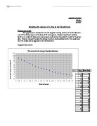
So to clarify how to get the values of these different function: one must select one of the optional items and then make sure to specify the data list names which are L1( press 2nd 1) and L2 ( press 2nd 2). It should be presented like this using the quadratic regression as an example:
Then to continue this assignment, each function shall be graphed using graphing programs such as Autograph or the calculator and evaluate which one suits the data best and why the others do not.
Linear function (ax+b)
This is function is probably the simplest to represent this data but it is the most inaccurate way. This graph tends to -∞ which is incorrect because there is no negative amount in the bloodstream.
A best fit line for this non-linear set of data would be one which tends to zero.
Quadratic function (ax² + bx + c)
This graph passes through points approximately but it is incorrect because of the fact that it doesn’t tend to 0 and instead shoots up to ∞.
Cubic Equation (ax³+bx²+cx+d)
The cubic equation resembles adequately to the behaviour of the non-linear data but it doesn’t suit it because like the linear equation it tends to -∞ which is incorrect because there is no negative amount in the bloodstream.
Exponential Function (abx )
This graph tends to zero, so therefore it cannot be a graph which tends to infinity like a cubic equation or a simple linear equation. This graph cannot start at -0 because there is no negative amounts in a bloodstream.
The quantity of drug tends to decrease over time at a rate proportional to its value, which would therefore mean it is an exponential function.
Note that it is an exponential decay, it never touches the x-axis, although it gets arbitrarily close to it (thus the x-axis is a horizontal asymptote to the graph).
Now that the function has been chosen, a question may have been asked on why this exponential function is formed as y=abx and does not look like y=ex (as it should popularly look like). The following explains why.
To start with, e is a mathematical constant, meaning it is a particular number or amount that never changes. In this case e is the base of the natural logarithm which equals approximately to 2.718281828.
When the exponential function is with a base of b it means this b = eλ where λ is equal to a constant.
The a which is placed before the b is f(0), which means it is the point where the graph cuts the y-axis.
If we put all these pieces the formula should evidently look like the following:
y=a(eλ )x
The calculator found the values for a and b of the exponential function using the least square fit, but it can also be found manually.
So in y = aeλx
-
a would be the initial quantity of drug administered. This therefore means it would be 10μg since it is the value of the y when x=0.
-
The value for x would be the time proportional to the amount of drug (y)
- λ can only be determined by factorising the equation the following way:
y = aeλx
y/a = eλx
λx = ln(y/a)
λ = ln(y/a)/x
Values for λ can be found for each proportional pairs, by substituting the x and y coordinates as shown in the example:
(x, y) = (0.5, 9) 9 = 10eλ0.5
9/10 = eλ0.5
λ0.5 = ln(9/10)
λ = ln(9/10)/0.5
= -0.211 3s.f.
The exponential function fits the non-linear data very well and corresponds well with the behaviour of the latter (although realistically time does not hold negative values). There are some differences between the coordinates of the exponential function and the coordinates of the non-linear data purely because a linear function cannot bear an accurate resemblance of a set of non-linear data. The function continues past 10 hours and estimates what happens to the amount of drug in the bloodstream as time continues to pass. This function is asymptotic, meaning that it never touches zero at the x-axis, although it gets arbitrarily. What this signifies is that the amount of drug in the bloodstream never disappears. This can be a legitimate statement: the amount of drug will be so small at some point that it will be impossible to trace, and therefore it would be considered that the person has no more amount of drug in his body.
Part B
In part B the patient is instructed to take a dosage of 10μg of this drug every 6 hours. A hypothesised diagram must be drawn out to show the drug in the bloodstream over a 24 hour period and state any assumptions made.
Then, using a graphing software (in this case Autograph) and the exponential model from part A, a model of an accurate graph must shown to represent this situation. Subsequently the maximum and the minimum amounts must be stated during this period.
Finally for the last step, a description must be achieved on what would happen to the found values over a following week if no further doses are taken and if doses are continued to being taken every six hours.
In the next page it shows an assumption of how the drug in the bloodstream behaves in the blood stream over a period of 24 hours. I assumed that the drug would get completely absorbed into the bloodstream after 6 hours before taking another dosage. It shows a regular steady increase but in fact realistically this assumption is incorrect because after 6 hours the amount of drug remaining from the previous drug intake is added to following drug intake. So hence this means that the amount after 6 hours would include residual amount of the previous doses.
So the functions for the 4 different graphs would be the following:
For 0≤ x <6 y = 10e-0.178x
For 6≤ x <12 y = 10e-0.178x + 10e-0.178(x-6)
For 12≤ x <18 y = 10e-0.178x + 10e-0.178(x-6)+ 10e-0.178(x-12)
For 18≤ x <24 y = 10e-0.178x + 10e-0.178(x-6)+ 10e-0.178(x-12) + 10e-0.178(x-18)
The coordinates of the functions where they intersect at the purple lines ( x=0, x=6, x=12, x=18, and x=24) should be recorded in order to find an average of the minimum and the maximum. They can be found by looking at the graph.
An average or mean is more accurate than a peak value because it is a result obtained by adding two or more amounts together and dividing the total by the number of amounts instead of looking at just one value (peak).
Note it is important to realise that the coordinates of the non-linear data will not be used, instead the data of the linear equation will.
( e.g. in the non-linear data when x=6 then y=3.7 but in the linear equation when x=6 then y=3.4)
To find the minimum amount during this period it is efficient to do an average of all the minimum values each six hours:
(3.4 + 4.6 + 5 + 5.2) ÷ 4
= 4.55
The minimum value is approximately 4.55μg
To find the maximum amount during this period an average is made (exactly like the minimum) for all values each six hours:
(13.4 + 14.6 + 15) ÷ 3
= 14.3333333
The minimum value is approximately 14.33333333μg
Realistically if no further doses were taken after this 24 hour period then the amount of drug in the bloodstream would decrease at the same rate as the initial function decreased, as there no new intake. Eventually there will be no drug left in the body. It could be argued abstractly though, that since it is an exponential decay, it never touches the x-axis, although it gets arbitrarily close to it (thus the x-axis is a horizontal asymptote to the graph). So according to the exponential function their will forever be some traces of drug in the body, but it would be so minute that realistically it would no longer be considered to be in the bloodstream for it could be difficult to identify.
If the drug is continued to be taken every six hours it would seem very predictable that the minimum and the maximum amount would eventually stabilize. The increase of each doses would decrease over time due to the exponential rate of decay. Hence this would clearly mean that the maximum and the minimum amount would tend to a stable value. The graph on the next page shows longer term behaviour over a 48 hour period, and this confirms my theory.
To make the maximum and minimum amounts more accurate I can find the average of the maximum and minimum of each graph:
Minimum
(3.4 + 4.6 + 5 + 5.2 + 5.2 + 5.2 + 5.2 + 5.2) ÷ 9
= 4.88
The minimum value is approximately 4.88μg
Maximum
(13.4 + 14.6 + 15 + 15.2 + 15.2 + 15.2 + 15.2) ÷ 7
= 14.8
The maximum value is approximately 14.8μg