Figure 2: The SIR model with rates of compartment change included
Where:
β – The rate at which an infected individual is able to make new infections from the susceptible compartment
γ – The rate at which an infected individual is able to recover and move into the removed compartment.
The SIR Model’s Differential Equations
As the SIR model is a compartmental model, with the rates depicting the ‘flow’ of individuals into each compartment, these rates can be expressed as differential equations:
Equation 1: The differential equation for S
This is the differential equation that represents the flow of individuals from the susceptible compartment into the Infected department. –βSI represents the rate of the ‘flow’. The equation is negative because individuals can only leave the S compartment to go into the I compartment and there are no other Susceptible individuals flowing in because of assumption (3).
Equation 2: The differential equation for I
This equation shows the rate at which susceptible individuals ‘flow in’ by becoming infected as βSI, minus the rate at which infected individuals recover and ‘flow out’,-γI into the Removed compartment.
Equation 3: The differential equation for R
This equation shows the rate at which Individuals recover from their infections and ‘flow’ from the Infected compartment to the Removed compartment as γI. As there are no other compartments for individuals to flow into after removed, there is no way that Removed individuals can leave the R compartment.
As stated before, the population equals the sum of the S, I and R compartments. This is because the sum of S’, I’ and R’ equals 0:
Equation 4: Proving that the sum of S, I and R is a constant.
When S’, I’ and R’ are summed, they all cancel out to 0, which indicates that the sum of the S, I and R compartments must be a constant, regardless of the fact that the S, I and R compartments are dynamic. This constant must therefore be the total population that is being studied, since the SIR model disregards the rate of births and deaths in the population that is being studied. This therefore derives the equation:
Equation 5: The sum of S, I and R
Information such as the duration of an epidemic or what effects a vaccination might have on an epidemic can be deduced from these differential equations. As the SIR model is a model of how a population, in fractions across each compartment, changes over time, these equations can be plotted on a line graph, but first they must be integrated. As mentioned before, these equations are all functions of t, for time in days.
The S – Susceptible equation
To simplify things, for the purpose of this integration, I will let a = βI
Where C is a constant as a result of this indefinite integration.
To calculate the constant, it’s necessary to think of what S would be at t = 0, that is before the epidemic broke out.
Since this particular equation is for when t = 0, the day before the epidemic broke out (where t = 1 is the first day of the epidemic), it can be assumed that the value at S when t = 0, would be N, the total population, as there would be no individuals in the I and R compartments and the equation for N is S + I + R. Thus, S at t = 0 can also be represented as S0
Because adding indices can only happen if their bases are being multiplied, the formula can be rewritten as:
Therefore,
Where:
β - The rate at which an infected individual is able to make new infections
I – The number of individuals in the infected compartment
t – Time in days
S0 – The number of susceptibles the day before the epidemic occurs, i.e. the total population.
Even though the integration is correct, we can immediately see a problem with this equation. Whilst β and S0 are constants, I is not a constant, since as stated before, it is a function of time, t and is therefore dynamic. As this equation is a function of t, t is the only number that can be variable, so I must use a different method to plot the graph of S. I can assume that since the equations for I’ and R’ include at least one of the other compartments, it would either not be possible or is at least outside of my scope of understanding for this level of mathematics to properly integrate I’ and R’.
An Alternative Method for Plotting the SIR model on a Graph
Earlier, I defined dS/dt as the rate of the ‘flow’ from the S compartment to the I compartment. It would be more correct to say that dS/dt is the rate of flow from the S compartment to the I compartment (dS) over a certain period of time (dt). With this definition, I can then employ Euler’s method to devise a simpler way of producing a line that is approximate to the line produced by the rate of change in the S compartment as the epidemic progresses. Remembering that S in the SIR model is a function of time, I can use this formula to produce a similar equation for S.
Formula taken from [http://en.wikipedia.org/wiki/Euler_method]
If we then assume that dS/dt can be written as:
Where:
dS/dt - -βSI
(n + 1) – Any time in the future
n – The present time
I can then rearrange this in terms S, which would give an approximate formula for the integration of dS/dt:
The same method applied to dI/dt devises the suitable formula for its approximate integration as well:
To keep the model simple, we can rely on the previous assumptions made about the SIR model. Since S + I + R = N, we can rearrange this to make R = N – S – I. When this is written in a similar form to the formulas above, we get:
Applying the SIR Model to the Re-Emerging H1N1 virus in Canada
The population of Canada is approximately 35,295,770. Within the population 8,292,255 is the estimated number of Canadians vaccinated against H1N1 since 2012. The Canadian government has a website called FluWatch, which collects data from all over Canada concerning the number of cases that crop up from each type of influenza strain. The very first case of H1N1 was detected on August 25th 2013 and FluWatch carefully monitors the number of H1N1 cases that are detected and publishes these numbers every week. I have been collecting these cases and have presented them in the following table:
Table 1: Number of H1N1 cases per week collected from FluWatch
By collecting the H1N1 cases from FluWatch, I have also been able to produce this graph:
Graph 1: A bar graph showing the number of H1N1 cases detected every week
To plot an SIR graph with this data, I need to establish what S0, I0, γ, dt and β are in relation to this particular case.
S0 is the number of susceptible individuals before the start of the epidemic. Since the population of Canada is 35,295,770 and there are 8,292,255 vaccinated Canadians, at the start of the epidemic there would be 27,003,515 susceptible individuals in the population.
We can find I0 by looking at the table of cases per week, in the first week, there were four cases of H1N1 detected. So, I0 in units per week would be 4, to find out the I0 in units per day, I would need to divide 4 by 7, which means that I0 in units per day is
One of the assumptions in the SIR model is that a fraction of the infected population recovers each day and moves from the infected compartment to the recovered compartment. This is represented as γ. Individuals that become infected by H1N1 will be infected for at least one day before symptoms show and subside. Symptoms of H1N1 typically last anywhere between 5 – 7 days, therefore an individual remains infectious for at most 8 days before they fully recover. Thus, for each day of the epidemic,
of the infected compartment recovers. The recovery rate, γ, is therefore:
The Basic Reproductive Number and β
Calculating β can be quite difficult, however we can estimate it what it might be by using the Basic Reproductive Number, represented as R0. The Basic Reproduction Number is defined as the number of infected individuals that one infected individual generates on average over the period of time that they are infected. The Basic Reproduction Number is used to determine whether a disease could cause an epidemic. If the R0 < 1, then a disease is not going to cause an epidemic. If R0 > 1, then the disease is epidemic. Typically, the higher the R0 number, the harder it is to control the spread of the disease.
There are two formulas which can be used to work out R0. One formula uses the average age at which the disease being studied is contracted in a static population, A, and the average life expectancy in said population. This is represented below:
A - The average age at which the disease is contracted in a given population.
L - The average life expectancy in a given population.
Calculating A – The Average Age of Canada
The table below, which was produced from data from the FluWatch website, shows cumulative data about the age of the individuals who contracted H1N1. I will be using this data to calculate what the average age of an individual who contracts H1N1 is.
Table 2 depicting the Cumulative H1N1 cases in Canada from Week 35 to Week 53 and calculating the average age, data taken from [ ]
Table 3 showing the mid-point(x) of each age group and product of the number of cases (f) with the mid-point (x). For the unknown age group, I used the mid-point between the age of an infant (0) and the average life expectancy in Canada (82.5)
Based on this calculation, the average age of an individual who contracts H1N1 is 35.62 years. The average life expectancy in Canada as of 2013 is 82.5, so L = 82.5.
Calculating R0 with the first formula
I can now use A = 35.62 and L = 82.5 to calculate the R0 of the re-emerging H1N1 virus in Canada.
The R0 for the H1N1 virus is estimated to be between 2 – 3, so I can assume my answer is relatively accurate, as it falls within 2 – 3.
Using the Basic Reproductive Number to Calculate β
The other formula to work out the R0 is given as:
Where:
β - The rate at which an infected individual is able to make new infections from the susceptible compartment.
– The average period of time an individual remains infectious, the reciprocal of the recovery rate.
Since
is the reciprocal of γ,
would be equal to 8. Now that I have the R0, 2.32, from the first formula, and the value for
, 8, I can rearrange the second formula to solve for β.
Applying the Calculated Values from the data on the SIR Model
To reiterate, the Euler Method formulas for the approximate integrations of S’ and I’ are:
To graph these formulas, we also need to know S0, I0, γ, dt and β.
S0 – 27,003,515
I0 -
γ -
β – 0.29
When these formulas and values are graphed, it looks like:
Graph 2: Graph produced based on Euler’s Method for approximate integration (appendix 1)
According to this model, the H1N1 virus epidemic would last for approximately 91 – 109 days. This is not a very accurate model, however as when it’s compared to the data of the number of infected cases collected from FluWatch, the number of infected cases do not match. Fortunately, I was able to find an excel sheet that generated a more accurate graph of what the expected SIR model would be, based on the same values I put in:
Graph 3: A more accurate graphical representation of the SIR model of H1N1 in Canada. The incubating period is just the amount of time an individual has the virus before they become contagious. For this graph, it’s possible to ignore the ‘incubating’ line, and the contagious line would be the same as a the ‘infected’ line. (Appendix 2)
According to this new graph, if a H1N1 epidemic broke out in Canada, it would last for approximately 77 days ±15 days (based on how each point was roughly selected), roughly 62 – 92 days. This was calculated by looking at the point where the susceptible population started to fall (the beginning of the epidemic):
And subtracting that value from the point where the recovered population converged with the value of the ‘Total Population’ again:
Vaccination and Herd Immunity with the Basic Reproduction Number
Now that I have predicted approximately how long the H1N1 epidemic would last for if it broke out, it is now worth looking into what could be done to hinder the epidemic or stop it altogether. Vaccinations are used to create a herd immunity within a population. Herd immunity is a type of immunity that arises when a certain percentage of a population has been immunised against a certain disease. The formula for herd immunity is given as:
Where q denotes the proportion of the population that is required to be vaccinated in order to achieve herd immunity. Since R0 was calculated earlier to be 2.32, this can then be solved as:
This therefore means that in order for Canada to develop a herd immunity against H1N1, at least 57% of the total population must be vaccinated. 57% of 35,292,770 is 20,118,589. As mentioned before, 8,292,255 Canadians are vaccinated against H1N1, thus at least 11,826,334 more Canadians must be vaccinated to achieve herd immunity against H1N1.
Conclusion and Reflection
I initially set out to:
- Predict if the re-emergence of H1N1 would cause an epidemic
- Plot the Epidemic as an SIR model
- Calculate the duration of the Epidemic
- Calculate the effects of Vaccination and how many individuals would need to be vaccinated to achieve a herd immunity.
Through this IA, I have been able to predict that based on current data, since the R0 is < 0 (R0 = 2.32), then the re-emergence of H1N1 is epidemic in Canada. My attempt at plotting this epidemic as an SIR model did not come out as planned, most likely due to my lack of understanding of the proper mathematics involved as they were outside the scope of my abilities, however I was able to produce a typical SIR graph with my calculated values in an SIR graph generator. By looking at the graph that was produced, I deduced that the epidemic would last anywhere between 66 – 92 days from the start. In order to achieve herd immunity, I calculated that 57% of the Canadian population must be vaccinated. With approximately 8.3m Canadians already vaccinated against this particular strain of the virus, more than 11.8m other Canadians must also be vaccinated to ensure herd immunity against H1N1.
The first thing worth talking about for my IA is that all of this work is based on the SIR model. Typically, a model is only as good as its assumptions, and since this is the simplest possible model within Epidemiology, it also makes unrealistic assumptions, such as the fact that a population is ‘static’ and unchanging. Of course, this is not true, as birth rates and death rates change the size of the population every single day. However, there are more sophisticated models that do account for the birth and death rates of a population, such as the SEIR model, as well as other highly variable factors that could be used. So, it’s entirely possible to calculate a more realistic model of the spread of the re-emerging H1N1 epidemic in Canada, it would just require a more in-depth understanding of the mathematics involved. Again, this is the very simplest model within Epidemiology that can be used, so it follows that this would also be the most unrealistic compared to subsequent models that account for other variables. There’s also the assumption that once an individual recovers from H1N1, they gain lifelong immunity to the virus and can no longer become infected again. Whilst this is true if it were the very same strain of H1N1, by nature, the pathogen is a virus, which means that it is highly adaptable and evolves at a much higher rate than other pathogens. Because of its high evolution rate, this means that theoretical, even if someone were immune to one version of H1N1, this would not guarantee that they are immune to a new, evolved version. The high adaptable of viral pathogens is specifically why new influenza vaccinations are developed each year for the ‘flu’ season.
Another limitation in this IA is that due to fact that the required understanding for this level of mathematics is far beyond my capabilities, I had to learn and use Euler’s method as a way of modelling this epidemic. Euler’s method in and of itself is only an approximation of the true graph that could be generated, which is another reason why this particular model is not as realistic as it could be. Regardless of these limitations, it does not mean that the SIR model and these calculations were completely pointless, as since they are estimations, they still point, in some regard to an approximate true model of the H1N1 epidemic. The purpose of Epidemiology is to predict the potential course of a disease, and by doing so, to devise appropriate counter-measures to hinder or stop it. By trying to understand the SIR model, I believe I have learned more about how diseases in general are spread and how these statistics and graphs are used to inform the public about the merits of vaccination. In the last couple of decades, the MMR vaccination scare has put many people off of vaccinating against Measles, Mumps and Rubella. However, with mathematical models such as the R0 number and subsequent SIR models, we are able to see that a lower vaccination rate would be disastrous for the population. Not only does a lower vaccination rate reduce the herd immunity and expose more vulnerable individuals, it also allows Measles, Mumps and Rubella time to evolve to withstand the vaccinations that were initially given out. This is precisely why mathematical models in epidemiology are needed. Research into more realistic mathematical models are what allow humans to effectively prepare for and stop potential epidemics, as well as to eradicate deadly diseases, like we have done with polio and almost with smallpox.
Appendices
Appendix 1 – Excel data used to produce Graph 2
Time(days) = B1
S(n) = C1
27003514.87 = C2
I(n) = D1
R(n) = E1
N = 35295770 = G1
γ = 8 = G5
β = 0.29 = G4
Excel Formula for S: =C2-($G$4/$G$1)*C2*D2
I: =D2+($G$4*C2*D2) - ($G$5*$G$3)
R: =$G$1-C3-D3
Appendix 2 – Model, Graph and Calculations for Graph 3
These are all available as an excel spreadsheet from
Bibliography
CTVNews. 2014. H1N1 virus: What you need to know. [online] Available at: http://www.ctvnews.ca/health/h1n1-virus-what-you-need-to-know-1.1609554 [Accessed: 13 Feb 2014].
Motivate.maths.org. 2014. Modelling with a spreadsheet | motivate.maths.org. [online] Available at: http://motivate.maths.org/content/DiseaseDynamics/Activities/Modelling [Accessed: 13 Feb 2014].
Oxforddictionaries.com. 2014. epidemiology: definition of epidemiology in Oxford dictionary (British & World English). [online] Available at: http://www.oxforddictionaries.com/definition/english/epidemiology [Accessed: 13 Feb 2014].
Phac-aspc.gc.ca. 2014. FluWatch report: December 29, 2013 to January 4, 2014 (Week 01) - Public Health Agency of Canada. [online] Available at: http://www.phac-aspc.gc.ca/fluwatch/13-14/w01_14/index-eng.php [Accessed: 13 Feb 2014].
Statcan.gc.ca. 2013. Statistics Canada: Canada's national statistical agency. [online] Available at: http://www.statcan.gc.ca/start-debut-eng.html [Accessed: 13 Feb 2014].
Statcan.gc.ca. 2013. Influenza immunization, less than one year ago by sex, by province and territory (Number). [online] Available at: http://statcan.gc.ca/tables-tableaux/sum-som/l01/cst01/health102a-eng.htm [Accessed: 13 Feb 2014].
Understand Seasonal Flu, Human Swine Flu and Hand-Foot-Mouth Diseases. 2014. [e-book] Hong Kong: Centre for Health Protection. p. 19. Available through: Centre for Health Protection http://www.chp.gov.hk/files/pdf/understand_seasonal_flu,_human_swine_flu_and_hand-foot-mouth_diseases_eng.pdf [Accessed: 13 Feb 2014].
Using Calculus to Model Epidemics. 2014. [e-book] Available through: homepage.math.uiowa.edu http://homepage.math.uiowa.edu/~stroyan/CTLC3rdEd/3rdCTLCText/Chapters/Ch2.pdf [Accessed: 13 Feb 2014].
Wikipedia. 2014. Epidemic model. [online] Available at: http://en.wikipedia.org/wiki/Epidemic_model [Accessed: 13 Feb 2014].
Wikipedia. 2014. Euler method. [online] Available at: http://en.wikipedia.org/wiki/Euler_method [Accessed: 13 Feb 2014].
Wikipedia. 2014. Basic reproduction number. [online] Available at: http://en.wikipedia.org/wiki/Basic_reproduction_number [Accessed: 13 Feb 2014].
Wikipedia. 2014. List of countries by life expectancy. [online] Available at: http://en.wikipedia.org/wiki/List_of_countries_by_life_expectancy#List_by_the_World_Health_Organization_.282013.29 [Accessed: 13 Feb 2014].
Wikipedia. 2014. Herd immunity. [online] Available at: http://en.wikipedia.org/wiki/Herd_immunity [Accessed: 13 Feb 2014].
Wikipedia. 2014. Mathematical modelling of infectious disease. [online] Available at: http://en.wikipedia.org/wiki/Mathematical_modelling_of_infectious_disease [Accessed: 13 Feb 2014].
http://www.ctvnews.ca/health/h1n1-virus-what-you-need-to-know-1.1609554
http://www.oxforddictionaries.com/definition/english/epidemiology
http://homepage.math.uiowa.edu/~stroyan/CTLC3rdEd/3rdCTLCText/Chapters/Ch2.pdf
http://en.wikipedia.org/wiki/Epidemic_model
http://en.wikipedia.org/wiki/Euler_method
http://www.statcan.gc.ca/start-debut-eng.html
http://statcan.gc.ca/tables-tableaux/sum-som/l01/cst01/health102a-eng.htm
http://en.wikipedia.org/wiki/Basic_reproduction_number
http://en.wikipedia.org/wiki/Mathematical_modelling_of_infectious_disease
http://en.wikipedia.org/wiki/List_of_countries_by_life_expectancy#List_by_the_World_Health_Organization_.282013.29
; http://www.chp.gov.hk/files/pdf/understand_seasonal_flu,_human_swine_flu_and_hand-foot-mouth_diseases_eng.pdf
http://motivate.maths.org/content/DiseaseDynamics/Activities/Modelling
http://en.wikipedia.org/wiki/Herd_immunity
http://en.wikipedia.org/wiki/Basic_reproduction_number