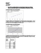
Mathematics 000065022 Mr. Hosington Kotaro Himi Use a GDC or graphing software to create data plot of speed versus thinking distance and data plot of speed versus braking distance. Describe your results. The data plot of speed versus thinking distance. The speed is relative to the thinking distance. So, this graph shows the direct proportion. There is no way that these values are minus because it doesn’t make sense that thinking distance is minus. In this report, let the time of stepping on the brake is equal. The data plot of speed versus braking distance.

The graph should show exponential function. It is conceivable that it causes friction when the car breaks. When the car starts breaking, the speed of car is on the table below. During the car keep breaking, speed is decreasing due to friction. Speed (km/h)Speed(m/s)00 328.8884813.336417.778022.229626.6611231.11 The relationship between the speed and advanced distance is shown the graph below. x = speed (m/s) y=advanced distance First, the speed of car is constant. Speed will be decreasing according to braking cause friction. Thus the advanced distance will be decreasing as well. At least, the car will stop which indicate point 0. Therefore, ...
This is a preview of the whole essay
The graph should show exponential function. It is conceivable that it causes friction when the car breaks. When the car starts breaking, the speed of car is on the table below. During the car keep breaking, speed is decreasing due to friction. Speed (km/h)Speed(m/s)00 328.8884813.336417.778022.229626.6611231.11 The relationship between the speed and advanced distance is shown the graph below. x = speed (m/s) y=advanced distance First, the speed of car is constant. Speed will be decreasing according to braking cause friction. Thus the advanced distance will be decreasing as well. At least, the car will stop which indicate point 0. Therefore, area of triangle represents braking distance (BD). Speed and distance are not constant because friction affects these aspects. BD = = = That’s why the relationship between speed and braking are exponential function. And, there is no way that exponential function through minus area because the car must not back when it is braking. Using your knowledge of functions, develop functions that model the behaviors noted in step 1. Speed (km/h)Thinking distance (m)Braking distance (m)3266489146412248015389618551122175 Speed versus thinking distance Speed versus thinking distance is linear function. Therefore, using [y = ax + b] a = slop b = intersect at y Substitute these values below into the function. Speed (km/h)Thinking distance (m)32648964128015961811221 x = speed y = thinking distance y = ax + b 6 = 32a + 0 32a = 6 a = y = x + b The value of b should be 0 because when the speed is 0, it is impossible to exist thinking time of trying to stop car. Therefore value of b has to be 0. Consequently the function will be; y = x This function is direct proportion thus all of values should be available. Now, check one of them. y= x y= 9 (thinking distance), x= 48 (speed) 9= ×48 9=9 As a result, this function is appropriate. The function is through all of the point thus this function is absolutely appropriate. Speed versus braking distance Speed versus braking distance is exponential function. Therefore, the appropriate equation will be; [y =]. Substitute these values below into the function to find the function. Speed (km/h)Braking distance (m)326481464248038965511275 x = speed y = braking thinking y= 6 = a= = = y= (0.00585) This is exponential function. The graph is almost through all of the point, but it is not absurdly correct. Now, check this function is appropriate. y= y=14 (braking distance), x=48(speed) 14=× 14= As a result, this function was not appropriate all value of table. It is conceivable that all of these value lead other function thus use the average of these function. ・When (x=48, y=14) 14= a a= = (0.00607) ・ When(x=64, y=24) 24= a a== (0.00583) ・ When (x=80,y=38) 38=a a= = (0.00593) ・When (x=96,y=55) 55=a a= = (0.00596) ・When (x=112,y=75) 75=a a== (0.00597) Thus the average value of a is able to calculate Average of a =・・・・・ =0.005998 Consequently, the function will be y=0.005998 Now, it is absurdly correct function which is able to show graph below. The overall stopping distance is obtained from adding the thinking distance to the braking distance. Create a data table of speed and overall stopping distance. Graph this data and describe the results. Speed (km/h)Stopping distance (m)3212482364368053967311296 Stopping distance is thinking distance add to breaking distance. x= speed y=stopping distance The graph is exponential function because overall stopping distance is that thinking distance add to braking distance that contain the aspect of friction. Tthis graph which is related between speed and overall distance is more sharp than other graph which is related speed and braking distance. The connection with braking distance and thinking distance is able to show on the graph below. Thinking distance is direct propotion. Braking distance is exponential function. And, overall stopping distance will be exponential function because stopping distance represent that thinking distance added to breaking distance which shows above. So, the function of overall stopping distance should be the curve which can draw through top of the bar graph. develop a function that models the relationship between speed and overall stopping distance. How is this function related to the functions obtained in step 2. Speed (km/h)Thinking distance (m)Braking distance (m)Stopping distance (m)3266124891423641224368015385396185573112217596 Find the function beteween speed and overall stopping distance. It can be find by using simultaneous equation and using the value of table. It is obvious that the function is quadorotic function. Therefore use [ y=+bx+c] to find the value of a, b, and c. Subsititu the value of the table above into the [y=+bx+c]. (x=speed y=stopping distance) 12= +32b+c…① 23= +48b+c…② 36= +64b+c…③ ②-① (23= +48b+c) - (12= +32b+c) = {(23-12) = (-) a+ (48-32) b} = {11= 1280 a+16b}…④ ③-② (36= +64b+c) – (23= +48b+c) = {(36-23) = (-) a+ (64-48) b} = { 13= 1792a+ 16b}…⑤ ⑤‐④ (13= 1792a+ 16b)- (11= 1280 a+16b) = {(13-11) = (1792-1280) a+ (16-16) b} = (2= 512a) = (512a=2) = (a=) = (a=) Substitute a= to ① and ② 12= +32b+c…⑥ 23= +48b+c…⑦ ⑦-⑥ (23= +48b+c)-( 12= +32b+c) =[(23-12) ={ ()-()}+ (48-32)b] = {11= (9-4)+16b} = {16b= (11-5)} = (b=) Substitute a and b to [12= +32b+c]…① 12= () + (32) +c 12= 4 + 12 +c c= 12-16 c= -4 Consequently, the function beteween speed and overall stopping distance is y= +x-4 It can be showed on the graph below. The first part of curve is through the appropriate points, but the end of curve has difference between curve and points. It might be caused by the value of (a) because overall stopping distance contain the braking distance. The speed is not constant during braking. Thus the value of (a) is not constant. The average of (a) will be draw appropriate curve. There is no way that overall stopping value will be minus. So, it is necessary to limit the available area of function. The intersection is 5 at x. Therefore (x>5). Anyway, this function is relationship between speed and overall stopping distance. Overall stopping distance represents thinking distance add to braking distance. It has a possibility that the function which has relationship between speed and stopping distance can be solve due to adding the both function that are thinking distance and braking distance which showed no2. Thinking distance y = Braking distance y=0.005998 (y=x)+(y=0.005998) = {2y=0.005998 +x} = (y= 0.01199+0.375x) That is certain wrong because that curve does not through any point. So the function which has value of a, b, and c is close to the appropriate curve. Overall stopping distance for other speeds and given below. Discuss how your model fits this data, and what modifications might be necessary. Speed (km/h)Stopping Distance (m)102.5 40179065160180 x= speed ,y=stipping distance This graph shows exportional function as well. Therefore it is possible to find the function according to use [y=+bx+c]. 2.5= a+10b+c…① 17= a+40b+c…② 65=a+90b+c…③ ②-① (17= a+40b+c)-(2.5= a+10b+c) ={(17-2.5)=( -)a+(40-10)b} =(14.5= 1500a+30b)…④ ③-② (65=a+90b+c)― (17= a+40b+c) = {(65-17) = (-) a+ (90-40) b} =(48=6500a+ 50b)…⑤ ⑤-④ (48=6500a+ 50b)-( 14.5= 1500a+30b) = {(144-72.5)=(19500-7500)a+(150-150)c} = (71.5=12000a) = (a= =0.00595) Substitute a value to ① and ② 2.5= ×+10b+c…⑥ 17= ×+40b+c…⑦ ⑦-⑥ (17= ×+40b+c)- (2.5= ×+10b+c) =[(17-2.5)= {(×)-( ×)}+ (40-10)b}] = (14.5= (9.53333-0.59583) +30b = (30b=14.5- 8.9375) = (b= =0.18541) Substitute value of a and b into the ① 2.5= ×+10×+c c=2.5-(0.59583+1.8541) c=2.5-2.44993=0.05007 Consequently, the function will be y=+x+0.05007 y=0.00595+0.18541x+0.05007 This function is fits the data table below. Speed (km/h)Stopping Distance (m)102.5 40179065160180 Moreover, this graph is fit other data as well. Speed (km/h)Stopping distance (m)3212482364368053967311296