AA is the approximated area for trapezium A, in units squared
AB is the approximated area for trapezium B, in units squared
AC is the approximated area for trapezium C, in units squared
AD is the approximated area for trapezium D, in units squared
AE is the approximated area for trapezium E, in units squared
Again an assumption must be made in regards to the length of the bases for each of the individual trapeziums. It is being postulated that, like before, the domain [0, 1] is divided equally between the five bases resulting in a length of 0.2 for each base.
TRAPEZIUM A [0, 0.2]:
-
h1: g(x) = x2 + 3
g(0) = (0)2 + 3
= 3
-
h2: g(x) = x2 + 3
g(0.2) = (0.2)2 + 3
= 3.04
-
b = 0.2
-
AA = (1/2) (b) (h1 + h2)
=(1/2) (0.2) (3 + 3.04)
= 0.604
TRAPEZIUM C [0.4, 0.6]:
-
h3: g(x) = x2 + 3
g(0.4) = (0.4)2 + 3
= 3.16
-
h4: g(x) = x2 + 3
g(0.6) = (0.6)2 + 3
= 3.36
-
b = 0.2
-
Ac = (1/2) (b) (h1 + h2)
=(1/2) (0.2) (3.16 + 3.36)
= 0.652
TRAPEZIUM E [0.8, 1.0]:
-
h5: g(x) = x2 + 3
g(0.8) = (0.8)2 + 3
= 3.64
-
h6: g(x) = x2 + 3
g(1.0) = (1.0)2 + 3
= 4.0
-
b = 0.2
-
Ac = (1/2) (b) (h1 + h2)
=(1/2) (0.2) (3.64 + 4.0)
= 0.764
TA= AA + AB + AC + AD + AE
TA= 0.604 + 0.62 + 0.652 + 0.7 + 0.764
TA= 3.34
With the help of technology, create diagrams showing and increasing number of trapeziums. For each diagram, find the approximation for the area. What do you notice?
Various diagrams will be created to depict the increasing number of trapeziums, which result in a greater precision for the approximation for the area.
First I calculated the area manually by hand. Then I tested these results with the use of technology, which in this case was the Riemann Sum Application on a TI-84+, which I used to create the table above.
The smaller the trapeziums, the more precise the area is because a smaller unit of measurement was utilized. It is possible to go on to infinity trapeziums, in which case the uncertainty would decrease more and more resulting in the relative error heading towards zero. This is because with more trapeziums it is possible to get a better approximation of the area since the line is going to a microscopic level, nearer to the original line. It gets nearer to the real value.
Use the diagram below to find a general expression for the area under the curve of g, from x = 0 to x = 1, using n trapeziums.
Based on the pattern observed from the diagrams above, a general equation can be written for the area under the curve of g, from x=0 to x=1, using n trapeziums. [g(x) = x2 + 3]
∫ca f(x) dx → ∫10 x2 + 3 dx
Where:
c is equal to the end x value of the domain
a is equal to the beginning x value for the domain
Y= f(x), the equation of the curve
dx indicates that everything is being taken in respects to x
The above equation in its expanded form is:
∫10 x2 + 3 dx = (1/2) b [g (0) + g (0.5)] + (1/2) b [g (0.5) + g (1)]
Where:
b is base which can be calculated by ( [c-a]/n )
This can be simplified to:
∫10 x2 + 3 dx = (1/2) b [g (0) + 2g (0.5) + g (1)]
For example, if the question with two trapeziums is solved using this formula:
g(x) = x2 + 3 from x = 0 to x = 1
∫10 = ½ b [g(x0) + g(x0.5)] + ½ h[g(x0.5) + g(x1)]
= ½ (0.5) (3 + 3.25) + ½ (0.5) (3.25 + 4)
= ½ (0.5) [3 + 4 + (2)(3.25)] = 3.375
Use your results to develop the general statement that will estimate the area under any curve y = f(x) from x = a to x = b using n trapeziums. Show clearly how you developed your statement.
∑ = ½ b [g(x0) + g(x1)] + ½ b [g(x1) + g(x2)] + ½ b [g(x2) + g(x3)] + ... + ½ b [g(xn-1) + (g(xn)]
b = ½ (c – a)/(n) = (c – a)/(2n) = (xn – x0)/(2n)
However, since b is a common factor it can be brought outside in a bracket. Also all the g(x) co-ordinates occur twice (in two consecutive trapeziums) apart from g(x0) and the last g(xn) co-ordinate. All the terms are halved which means the first and last g(x) values are halved and every other g(x) value should be counted once.
This can be re-written to, if using n trapeziums:
∫ca f(x) dx =(1/2) b [g(x0) + g(xn)+ 2(g(x1)+ g(x2)+ g(x3)+ . . . + g(xn-1)]
∫ca f(x) dx = [(xn – x0)/(2n)] (g(x0) + g(xn) + 2[∑ g(xi)])
Where:
n is the number of trapeziums the area of the curve is divided into
b is base which can be calculated by ( [c-a]/n )
c is equal to 1 in this problem or (xn)
a is equal to 0 in this question or (x0)
g(x0)… g(xn) are the y values for each respective x value.
Use your general statement, with eight trapeziums, to find approximations for these areas.
∫ca (x/2)^(2/3) dx = (xn – x0)/(2n) (g(x0) + g(xn) + 2[∑ g(xi)]
∫31(x/2)^(2/3) dx =(3-1)/(2x8) (g(3) + g(1) + 2[g(1.25) + g(1.5) + g(1.75) + g(2) + g(2.25) + g(2.5) + g(2.75)]
= (2)/(16)[0.63 + 1.31 + 2 (0.73 + 0.83 + 0.91 + 1 + 1.08 + 1.16 + 1.24)]
=1.98
∫ca (9x)/ (√x3 + 9) dx = (xn – x0)/(2n) (g(x0) + g(xn) + 2[∑ g(xi)]
∫31(9x)/ (√x3 + 9) dx =(2)/(16) (g(3) + g(1) + 2[g(1.25) + g(1.5) + g(1.75) + g(2) + g(2.25) + g(2.5) + g(2.75)]
= (2)/(16)[2.85 + 4.5 + 2 (3.40 + 3.84 + 4.16 + 4.37 + 4.48 + 4.53 + 4.54)]
= 8.24625
∫ca (9x)/ (√x3 + 9) dx = (xn – x0)/(2n) (g(x0) + g(xn) + 2[∑ g(xi)]
∫31(4x3 – 23x2 + 40x - 18)dx =(2)/(16) (g(3) + g(1) + 2[g(1.25)+g(1.5)+g(1.75)+g(2)+g(2.25)+g(2.5)+g(2.75)]
= (2)/(16)( [3 + 3 + 2(3.875 + 3.75 + 3 + 2 + 1.125 + 0.75 + 1.25)]
= 4.6875
Find and compare these answers with your approximations. Comment on the accuracy of your approximations.
KEY STROKES: math-> 9. fnInt ( enter equation ,X ,1 ,3 ) ENTER
∫f(x) dx = 1.9806909
∫f(x) dx = 8.2597312
∫f(x) dx = 4.6666667
The approximated results that were achieved by manual calculation were very precise from the actual area underneath the curve. Based on the equation, the percent of variation changes; however, the data is precise at least up to the tenths place.
Use other functions to explore the scope and limitations of your general statement. Does it always work? Discuss how the shape of a graph influences your approximation.
For each function n=4 trapeziums and the interval is [0,1], and [(xn – x0)/ (2n)] = (1/8)
-
y = x4 + 12x + 4
∫ca f(x) dx = [(xn – x0)/(2n)] (g(x0) + g(xn) + 2[∑ g(xi)])
x0 : g(x) = x4 + 12x + 4
g(0) = (0)4 + 12(0) + 4
= 4
xn : g(x) = x4 + 12x + 4
g(1) = (1)4 + 12(1) + 4
= 17
∫10 (x4 + 12x + 4) dx = (1/8) (4 + 17 + 2[7.00390625 + 10.0625 + 13.31640625]
= 10.22070313
Calculator:
math-> 9. fnInt ( enter x4 + 12x +4 ,X ,1 ,3 ) ENTER OR Y= enter y = x4 + 12x + 4 2nd TRACE 7 ENTER graph displayed 0 ENTER 1 S ENTER S
∫f(x)dx = 10.2
-
y = x3 + 10
∫ca f(x) dx = [(xn – x0)/(2n)] (g(x0) + g(xn) + 2[∑ g(xi)])
x0 : g(x) = x3 + 10
g(0) = (0)3 + 10
= 10
xn : g(x) = x3 + 10
g(1) = (1)3 + 10
= 11
∫10 (x3 + 10) dx = (1/8) (10 + 11 + 2[10.015625 + 10.000125 + 10.421875]
= 10.23440625
Calculator:
math-> 9. fnInt ( enter x3 + 10 ,X ,1 ,3 ) ENTER OR Y= enter y = x3 + 10 2nd TRACE 7 ENTER graph displayed 0 ENTER 1 S ENTER S
∫f(x)dx = 10.25
-
y = 2/(x2 + 4)
∫ca f(x) dx = [(xn – x0)/(2n)] (g(x0) + g(xn) + 2[∑ g(xi)])
x0 : g(x) = 2/(x2 + 4)
g(0) = 2/(02 + 4)
= 0.5
xn : g(x) = 2/(x2 + 4)
g(1) = 2/(12 + 4)
= 0.4
∫10 (2/(x2 + 4)) dx = (1/8) (0.5 + 0.4 + 2[0.4923076923+ 0.4705882353+ 0.4383561644]
= 0.462813023
Calculator:
math-> 9. fnInt ( enter 2/(x2 + 4) ,X ,1 ,3 ) ENTER OR Y= enter y = 2/(x2 + 4) 2nd TRACE 7 ENTER graph displayed 0 ENTER 1 S ENTER S
∫f(x)dx = 0.463647609
-
y = √(2x+1)
∫ca f(x) dx = [(xn – x0)/(2n)] (g(x0) + g(xn) + 2[∑ g(xi)])
x0 : g(x) = √(2x+1)
g(0) = √(2(0)+1)
= 1
xn : g(x) = √(2x+1)
g(1) = √(2(1)+1)
= 1.732050808
∫10 (√(2x+1)) dx = (1/8) (1 + 1.73 + 2[1.224744871 + 1.414213562 + 1.58113883]
= 1.396530667
Calculator:
math-> 9. fnInt ( enter 2/(x2 + 4) ,X ,1 ,3 ) ENTER OR Y= enter y = 2/(x2 + 4) 2nd TRACE 7 ENTER graph displayed 0 ENTER 1 S ENTER S
∫f(x)dx = 1.398717474
CONCLUSION
The manual calculations derived from the general statement appeared to be very close to the exact answers as computed by the calculator. Based on the results, it appears that no matter the shape, using the trapezium rule provides with a fairly accurate and precise approximation.
However, it can be determined in two ways whether the approximation is an overestimate or an underestimate. The first is to sketch a graph and draw the trapeziums. If the tops of the trapeziums are above the curve, there is an overestimate, and if the trapeziums are below the curve, it is an underestimate. The second method is to examine the second derivative of the graph. If it is negative, indicating concave down, then the curve will have a lesser gradient at any given interval in the positive x-direction, and therefore the trapeziums will be underneath the curve. If the second derivative is positive, indicating upwards concavity, trapeziums will extrude, and thus give an overestimate.
Overall, to achieve the most precise and accurate approximation for an area under the curve, n, the number of trapeziums, needs to be divided into smaller subintervals.